graph TD
    A[Chi-square Test and Other<br/>Non-parametric Tests] --> B[Chi-square χ²]
    A --> C[Other non-parametric<br/>tests]

    B --> B1[Goodness of fit]
    B --> B2[Test of independence]

    B1 --> B1a[Uniform distribution]
    B1 --> B1b[A specific pattern]
    B1 --> B1c[Normal distribution]

    C --> C1[Sign test]
    C --> C2[Runs test]
    C --> C3[Mann-Whitney test]
    C --> C4[Spearman rank<br/>correlation]
    C --> C5[Kruskal-Wallis test]
15 Chi-square Test and Other Non-parametric Tests
15.1 Chapter Overview
This chapter introduces statistical tests that do not require assumptions about population parameters or distributions. While previous chapters relied on parametric tests (requiring normal distributions or specific variance patterns), non-parametric tests provide robust alternatives when such assumptions cannot be made.
We explore the chi-square (\chi^2) test for goodness of fit and independence, along with other distribution-free methods including the sign test, runs test, Mann-Whitney U test, Spearman rank correlation, and Kruskal-Wallis test.
15.2 Business Scenario: Mama’s Pizzeria
15.3 14.1 Introduction to Non-parametric Tests
Previous chapters presented numerous hypothesis tests for population means and proportions. Some required large samples (n > 30), while others worked with small samples. We examined tests for single populations and comparative tests across multiple populations.
However, all these testing situations shared one common characteristic: they required certain assumptions about the population. For example:
- t-tests required the assumption that the population was normally distributed
- F-tests required assumptions about variance patterns
- z-tests relied on known population parameters or large sample sizes
Because such tests depend on postulates about the population and its parameters, they are called parametric tests.
ImportantWhen Parametric Assumptions Fail
In practice, many business situations arise where it is simply not possible to safely make assumptions about:
- The value of a population parameter
- The form of the population distribution
When parametric test assumptions cannot be met, most tests described in previous chapters become inapplicable.
15.3.1 Non-parametric Tests: Distribution-Free Methods
Non-parametric tests (also called distribution-free tests) provide alternatives that do not depend on:
- A single type of distribution
- Specific parameter values
TipDefinition: Non-parametric Tests
Non-parametric tests are statistical procedures that can be used to test hypotheses when assumptions about population parameters or distributions are not possible or cannot be verified.
Key advantages:
- No normality assumptions required
- Robust to outliers and skewed distributions
- Applicable to ordinal and nominal data
- Often based on ranks rather than actual values
15.4 14.2 The Chi-square (\chi^2) Distribution
One of the most useful non-parametric tools is the chi-square test (\chi^2). Like the t-distribution, the chi-square distribution is actually a family of distributions—there exists a different chi-square distribution for each degree of freedom.
15.4.1 Properties of the Chi-square Distribution
Code
import numpy as np
import matplotlib.pyplot as plt
from scipy.stats import chi2

# Create x values
x = np.linspace(0, 20, 500)

# Different degrees of freedom
df_values = [1, 2, 3, 5, 10]
colors = ['#D62828', '#F77F00', '#FCBF49', '#2E86AB', '#06A77D']

fig, ax = plt.subplots(figsize=(12, 7))

for df, color in zip(df_values, colors):
    y = chi2.pdf(x, df)
    ax.plot(x, y, linewidth=2.5, label=f'df = {df}', color=color)

ax.set_xlabel('χ² Value', fontsize=13, fontweight='bold')
ax.set_ylabel('Probability Density', fontsize=13, fontweight='bold')
ax.set_title('Chi-square Distribution: Less Skewed as df Increases',
             fontsize=14, fontweight='bold', pad=20)
ax.legend(fontsize=11, loc='upper right')
ax.grid(True, alpha=0.3, linestyle='--')
ax.set_xlim(0, 20)
ax.set_ylim(0, 0.5)

plt.tight_layout()
plt.show()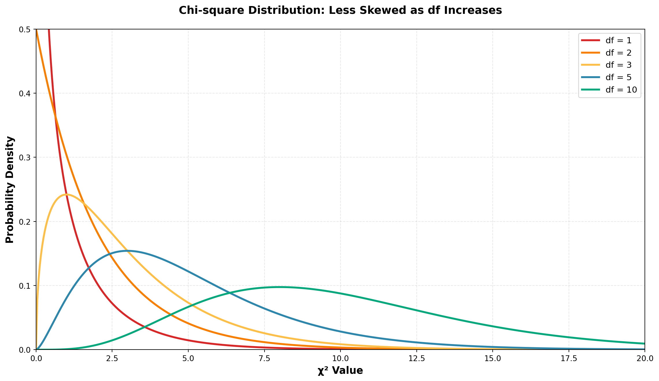
NoteKey Observation
As the number of degrees of freedom increases, the chi-square distribution becomes less skewed and more symmetric. With higher df values, the distribution begins to resemble a normal distribution.
15.4.2 Two Primary Applications of Chi-square Tests
The chi-square test has two most common applications:
- Goodness of Fit Tests — Testing whether sample data fits a hypothesized distribution pattern
- Tests of Independence — Testing whether two categorical variables are independent
We will examine each application in detail.
15.5 14.3 Goodness of Fit Tests
Business decisions frequently require testing hypotheses about unknown population distributions. For example, we might hypothesize that:
- The population distribution is uniform (all values equally likely)
- The population follows a specific pattern (e.g., 60% category A, 30% category B, 10% category C)
- The population is normally distributed
The hypotheses would be stated as:
\begin{aligned} H_0 &: \text{The population distribution follows the hypothesized form} \\ H_A &: \text{The population distribution does NOT follow the hypothesized form} \end{aligned}
TipDefinition: Goodness of Fit Test
A goodness of fit test measures how closely observed sample data fits a particular hypothesized distribution form. If the fit is reasonably close, we can conclude that the hypothesized distribution exists.
Decision logic:
- Large differences between observed and expected frequencies → Reject H_0
- Small differences (attributable to sampling error) → Do not reject H_0
15.5.1 The Chi-square Test Statistic
The chi-square goodness of fit test determines whether sample observations “fit” expectations based on the hypothesized distribution.
Chi-square Test Formula:
\chi^2 = \sum_{i=1}^{K} \frac{(O_i - E_i)^2}{E_i} \tag{15.1}
Where:
- O_i = Observed frequency of events in the sample data
- E_i = Expected frequency of events if H_0 is true
- K = Number of categories or classes
Degrees of Freedom:
df = K - m - 1
Where:
- K = Number of categories
- m = Number of parameters estimated from the data
ImportantUnderstanding the Test Statistic
The numerator (O_i - E_i)^2 measures the squared difference between observed and expected frequencies.
Interpretation:
- Large differences → Large \chi^2 value → Reject H_0
- Small differences → Small \chi^2 value → Do not reject H_0
The chi-square test is always a right-tailed test because we’re looking for large deviations from expectations.
15.5.2 Example: Testing for Uniform Distribution
Scenario: Chris Columbus, Marketing Director at Seven Seas, Inc., manages inventory for four types of boats sold by the firm. He has historically ordered new boats assuming the four types are equally popular with uniform demand.
However, inventory control has become more difficult recently, prompting Chris to test his uniformity assumption.
Hypotheses:
\begin{aligned}
H_0 &: \text{Demand is uniform across all four boat types} \\
H_A &: \text{Demand is NOT uniform across all four boat types}
\end{aligned}
Data Collection:
Chris selects a random sample of n = 48 boats sold during recent months.
Expected Frequencies:
If demand is truly uniform, he would expect: E_i = \frac{48}{4} = 12 boats of each type sold.
Observed vs. Expected:
| Boat Type | Observed Sales (O_i) | Expected Sales (E_i) |
|---|---|---|
| Pirates’ Revenge | 15 | 12 |
| Jolly Roger | 11 | 12 |
| Bluebeard’s Treasure | 10 | 12 |
| Ahab’s Quest | 12 | 12 |
| Total | 48 | 48 |
NoteImportant Property
Note that \sum O_i = \sum E_i = 48. The total observed frequencies must always equal the total expected frequencies.
Calculating the Test Statistic:
Using Equation 15.1:
\begin{aligned} \chi^2 &= \frac{(15-12)^2}{12} + \frac{(11-12)^2}{12} + \frac{(10-12)^2}{12} + \frac{(12-12)^2}{12} \\[10pt] &= \frac{9}{12} + \frac{1}{12} + \frac{4}{12} + \frac{0}{12} \\[10pt] &= \frac{14}{12} \\[10pt] &= 1.17 \end{aligned}
Degrees of Freedom:
- No parameters need to be estimated, so m = 0
- df = K - m - 1 = 4 - 0 - 1 = 3
Critical Value:
At \alpha = 0.05 with df = 3, from the chi-square table:
\chi^2_{0.05, 3} = 7.815
Decision Rule:
- Do not reject H_0 if \chi^2 \leq 7.815
- Reject H_0 if \chi^2 > 7.815
Code
import numpy as np
import matplotlib.pyplot as plt
from scipy.stats import chi2

# Set up the distribution
df = 3
x = np.linspace(0, 15, 500)
y = chi2.pdf(x, df)

# Critical value and test statistic
critical_value = 7.815
test_statistic = 1.17

fig, ax = plt.subplots(figsize=(12, 7))

# Plot the distribution
ax.plot(x, y, linewidth=3, color='#2E86AB', label='χ² distribution (df=3)')

# Fill critical region
x_crit = x[x >= critical_value]
y_crit = chi2.pdf(x_crit, df)
ax.fill_between(x_crit, y_crit, alpha=0.3, color='#D62828',
                 label=f'Rejection region (α = 0.05)')

# Mark critical value
ax.axvline(critical_value, color='#D62828', linestyle='--', linewidth=2.5,
           label=f'Critical value = {critical_value}')

# Mark test statistic
ax.axvline(test_statistic, color='#06A77D', linestyle='-', linewidth=3,
           label=f'Test statistic χ² = {test_statistic}')
ax.plot(test_statistic, chi2.pdf(test_statistic, df), 'o',
        markersize=12, color='#06A77D', zorder=5)

ax.set_xlabel('χ² Value', fontsize=13, fontweight='bold')
ax.set_ylabel('Probability Density', fontsize=13, fontweight='bold')
ax.set_title('Chi-square Goodness of Fit Test: Seven Seas Boat Sales',
             fontsize=14, fontweight='bold', pad=20)
ax.legend(fontsize=11, loc='upper right')
ax.grid(True, alpha=0.3, linestyle='--')
ax.set_xlim(0, 15)

plt.tight_layout()
plt.show()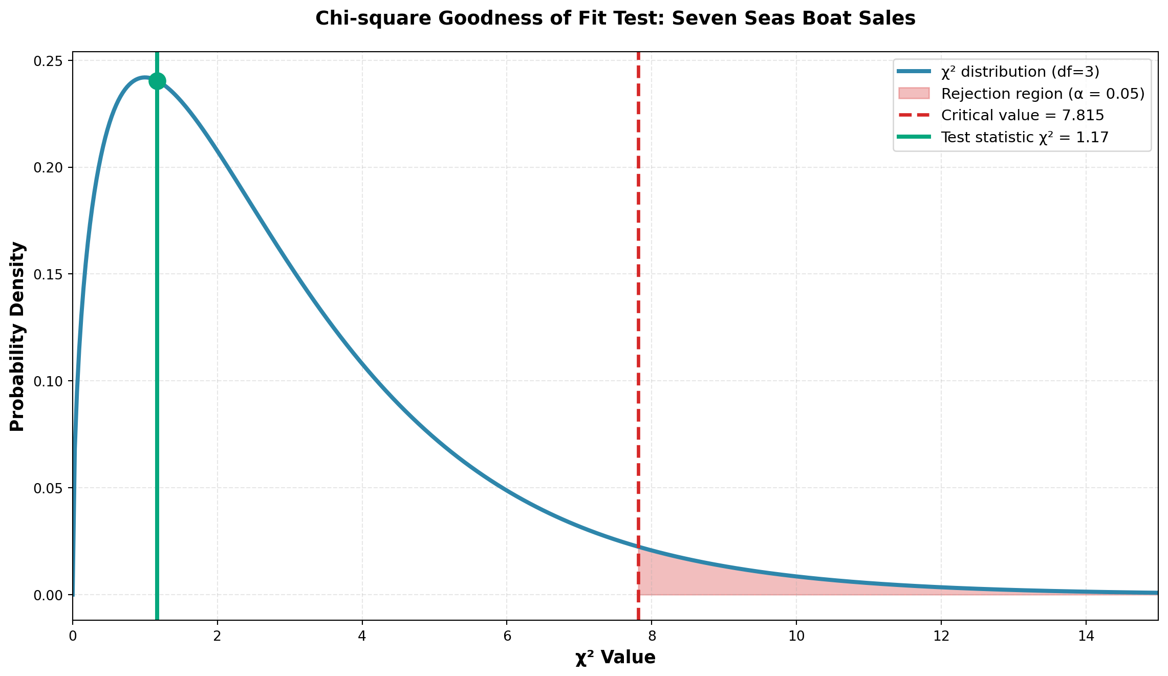
Conclusion:
Since \chi^2 = 1.17 < 7.815 (critical value), we do not reject H_0.
NoteInterpretation
The differences between what was actually observed (O_i) and what Chris expected under uniform demand (E_i) are not large enough to refute the null hypothesis. The differences are not statistically significant and can be attributed simply to sampling error.
Business implication: Chris can continue his inventory ordering policy based on uniform demand across the four boat types.
P-value:
The p-value for this test is the area to the right of \chi^2 = 1.17 under the chi-square distribution with df = 3.
Code
from scipy.stats import chi2

# Calculate p-value
test_stat = 1.17
df = 3
p_value = 1 - chi2.cdf(test_stat, df)

print(f"Test statistic: χ² = {test_stat}")
print(f"Degrees of freedom: df = {df}")
print(f"P-value = {p_value:.4f}")
print(f"\nSince p-value ({p_value:.4f}) > α (0.05), we do not reject H₀")
Test statistic: χ² = 1.17
Degrees of freedom: df = 3
P-value = 0.7602
Since p-value (0.7602) > α (0.05), we do not reject H₀The p-value of approximately 0.76 is much greater than \alpha = 0.05, confirming our decision to not reject the null hypothesis.
15.6 14.4 Testing for a Specific Pattern
In the Seven Seas example, Chris assumed equal demand across all four boat types, resulting in identical expected frequencies. However, many business situations involve testing against a specific pattern where expected frequencies are not all equal.
In such cases, expected frequencies must be calculated as:
Expected Frequency Formula:
E_i = n \cdot p_i {#eq-expected-freq}
Where:
- n = sample size
- p_i = probability of each category as specified in H_0
15.6.1 Example: John Dillinger First National Bank
Scenario: The John Dillinger First National Bank in New York follows a lending policy to extend:
- 60% of loans to commercial businesses
- 10% of loans to individuals
- 30% of loans to foreign borrowers
Jay Hoover, Vice President of Marketing, wants to determine whether this policy is being maintained.
Sample: He randomly selects 85 recently approved loans and finds:
- 62 loans to businesses
- 10 loans to individuals
- 13 loans to foreign borrowers
Hypotheses:
\begin{aligned}
H_0 &: \text{The desired pattern is maintained: 60\% commercial, 10\% personal, 30\% foreign} \\
H_A &: \text{The desired pattern is NOT maintained}
\end{aligned}
Calculating Expected Frequencies:
If H_0 is true, Mr. Hoover would expect:
- Commercial loans: E_1 = (85)(0.60) = 51.0 loans
- Personal loans: E_2 = (85)(0.10) = 8.5 loans
- Foreign loans: E_3 = (85)(0.30) = 25.5 loans
Data Summary:
| Loan Type | Observed Frequency (O_i) | Expected Frequency (E_i) |
|---|---|---|
| Commercial | 62 | 51.0 |
| Personal | 10 | 8.5 |
| Foreign | 13 | 25.5 |
| Total | 85 | 85.0 |
Calculating Chi-square:
\begin{aligned} \chi^2 &= \frac{(62-51)^2}{51} + \frac{(10-8.5)^2}{8.5} + \frac{(13-25.5)^2}{25.5} \\[10pt] &= \frac{121}{51} + \frac{2.25}{8.5} + \frac{156.25}{25.5} \\[10pt] &= 2.37 + 0.26 + 6.13 \\[10pt] &= 8.76 \end{aligned}
Test Parameters:
- No parameters estimated: m = 0
- Categories: K = 3
- Degrees of freedom: df = K - m - 1 = 3 - 0 - 1 = 2
- Significance level: \alpha = 0.10
- Critical value: \chi^2_{0.10, 2} = 4.605
Decision Rule:
- Do not reject H_0 if \chi^2 \leq 4.605
- Reject H_0 if \chi^2 > 4.605
Code
import numpy as np
import matplotlib.pyplot as plt
from scipy.stats import chi2

# Test parameters
df = 2
test_statistic = 8.76
critical_value = 4.605
alpha = 0.10

# Create distribution
x = np.linspace(0, 15, 500)
y = chi2.pdf(x, df)

fig, ax = plt.subplots(figsize=(12, 7))

# Plot distribution
ax.plot(x, y, linewidth=3, color='#2E86AB', label=f'χ² distribution (df={df})')

# Fill rejection region
x_reject = x[x >= critical_value]
y_reject = chi2.pdf(x_reject, df)
ax.fill_between(x_reject, y_reject, alpha=0.3, color='#D62828',
                 label=f'Rejection region (α = {alpha})')

# Mark critical value
ax.axvline(critical_value, color='#D62828', linestyle='--', linewidth=2.5,
           label=f'Critical value = {critical_value}')

# Mark test statistic
ax.axvline(test_statistic, color='#F77F00', linestyle='-', linewidth=3,
           label=f'Test statistic χ² = {test_statistic}')
ax.plot(test_statistic, chi2.pdf(test_statistic, df), 'o',
        markersize=14, color='#F77F00', zorder=5)

# Add annotation
ax.annotate('REJECT H₀', xy=(test_statistic, chi2.pdf(test_statistic, df)),
            xytext=(test_statistic + 2, 0.15),
            fontsize=12, fontweight='bold', color='#D62828',
            arrowprops=dict(arrowstyle='->', color='#D62828', lw=2))

ax.set_xlabel('χ² Value', fontsize=13, fontweight='bold')
ax.set_ylabel('Probability Density', fontsize=13, fontweight='bold')
ax.set_title('Chi-square Test: Bank Loan Portfolio Compliance',
             fontsize=14, fontweight='bold', pad=20)
ax.legend(fontsize=11, loc='upper right')
ax.grid(True, alpha=0.3, linestyle='--')
ax.set_xlim(0, 15)

plt.tight_layout()
plt.show()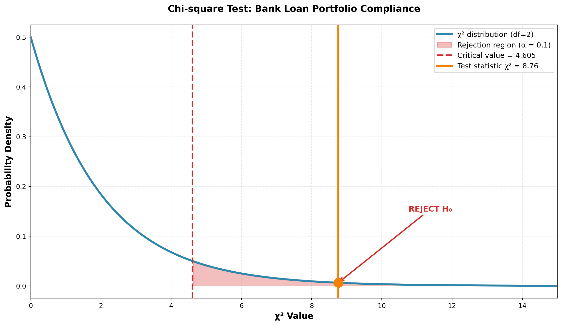
Conclusion:
Since \chi^2 = 8.76 > 4.605 (critical value), we reject H_0.
ImportantInterpretation
The differences between what Mr. Hoover observed and what he expected under the desired loan portfolio pattern are too large to be attributed to chance alone.
There is only a 10% probability that a random sample of 85 loans could produce the observed frequencies if the bank were actually maintaining its desired lending pattern.
Business implication: The bank is NOT following its stated 60%-10%-30% lending policy. Management should investigate why the actual distribution (73% commercial, 12% personal, 15% foreign) deviates significantly from policy, particularly the shortfall in foreign loans.
15.7 14.5 Testing for Normality
15.7.1 Aqua Lung Scuba Tank Example
Scenario: Production specifications for scuba diving air tanks require:
- Mean pressure: \mu = 600 psi
- Standard deviation: \sigma = 10 psi
- Distribution: Must be normally distributed for safety
You have just been hired by Aqua Lung, a major manufacturer of diving equipment. Your first task is to determine whether fill levels follow a normal distribution.
Aqua Lung is confident that \mu = 600 psi and \sigma = 10 psi are maintained. Only the nature of the distribution needs testing.
Hypotheses:
\begin{aligned}
H_0 &: \text{Fill levels are normally distributed} \\
H_A &: \text{Fill levels are NOT normally distributed}
\end{aligned}
Sample: n = 1000 tanks measured, producing the following distribution:
| PSI Range | Observed Frequency (O_i) |
|---|---|
| Below 580 | 20 |
| 580 to < 590 | 142 |
| 590 to < 600 | 310 |
| 600 to < 610 | 370 |
| 610 to < 620 | 128 |
| 620 and above | 30 |
| Total | 1000 |
15.7.2 Calculating Expected Frequencies Under Normality
To determine expected frequencies, calculate the probability that a randomly selected tank falls in each interval, assuming N(600, 10).
Example for first interval: P(X < 580)
Z = \frac{580 - 600}{10} = -2.0
From the standard normal table: P(Z < -2.0) = 0.0228
Therefore: E_1 = (1000)(0.0228) = 22.8 tanks
Example for second interval: P(580 < X < 590)
\begin{aligned} Z_1 &= \frac{580 - 600}{10} = -2.0 \quad \text{(area = 0.4772)} \\[8pt] Z_2 &= \frac{590 - 600}{10} = -1.0 \quad \text{(area = 0.3413)} \end{aligned}
Therefore: P(580 < X < 590) = 0.4772 - 0.3413 = 0.1359
Expected frequency: E_2 = (1000)(0.1359) = 135.9 tanks
Code
import numpy as np
import matplotlib.pyplot as plt
from scipy.stats import norm

fig, axes = plt.subplots(1, 3, figsize=(16, 5))

mu, sigma = 600, 10
x = np.linspace(560, 640, 500)
y = norm.pdf(x, mu, sigma)

# Panel 1: P(X < 580)
ax = axes[0]
ax.plot(x, y, linewidth=2.5, color='#2E86AB')
x_fill = x[x < 580]
y_fill = norm.pdf(x_fill, mu, sigma)
ax.fill_between(x_fill, y_fill, alpha=0.4, color='#D62828')
ax.axvline(580, color='#D62828', linestyle='--', linewidth=2)
ax.text(570, 0.025, 'P(X < 580)\n= 0.0228', fontsize=11,
        bbox=dict(boxstyle='round', facecolor='wheat', alpha=0.8))
ax.set_xlabel('PSI', fontsize=11, fontweight='bold')
ax.set_ylabel('Probability Density', fontsize=11, fontweight='bold')
ax.set_title('Area Below 580 psi', fontsize=12, fontweight='bold')
ax.grid(True, alpha=0.3)

# Panel 2: P(580 < X < 590)
ax = axes[1]
ax.plot(x, y, linewidth=2.5, color='#2E86AB')
x_fill = x[(x >= 580) & (x < 590)]
y_fill = norm.pdf(x_fill, mu, sigma)
ax.fill_between(x_fill, y_fill, alpha=0.4, color='#F77F00')
ax.axvline(580, color='#F77F00', linestyle='--', linewidth=2)
ax.axvline(590, color='#F77F00', linestyle='--', linewidth=2)
ax.text(585, 0.025, 'P(580 < X < 590)\n= 0.1359', fontsize=11,
        bbox=dict(boxstyle='round', facecolor='wheat', alpha=0.8))
ax.set_xlabel('PSI', fontsize=11, fontweight='bold')
ax.set_title('Area Between 580-590 psi', fontsize=12, fontweight='bold')
ax.grid(True, alpha=0.3)

# Panel 3: Symmetric distribution
ax = axes[2]
ax.plot(x, y, linewidth=2.5, color='#2E86AB', label='N(600, 10)')
# Mark all intervals
intervals = [580, 590, 600, 610, 620]
for interval_val in intervals:
    ax.axvline(interval_val, color='gray', linestyle=':', linewidth=1.5, alpha=0.7)
ax.axvline(600, color='#06A77D', linestyle='-', linewidth=2.5, label='μ = 600')
ax.set_xlabel('PSI', fontsize=11, fontweight='bold')
ax.set_title('Complete Normal Distribution', fontsize=12, fontweight='bold')
ax.legend(fontsize=10)
ax.grid(True, alpha=0.3)

plt.tight_layout()
plt.show()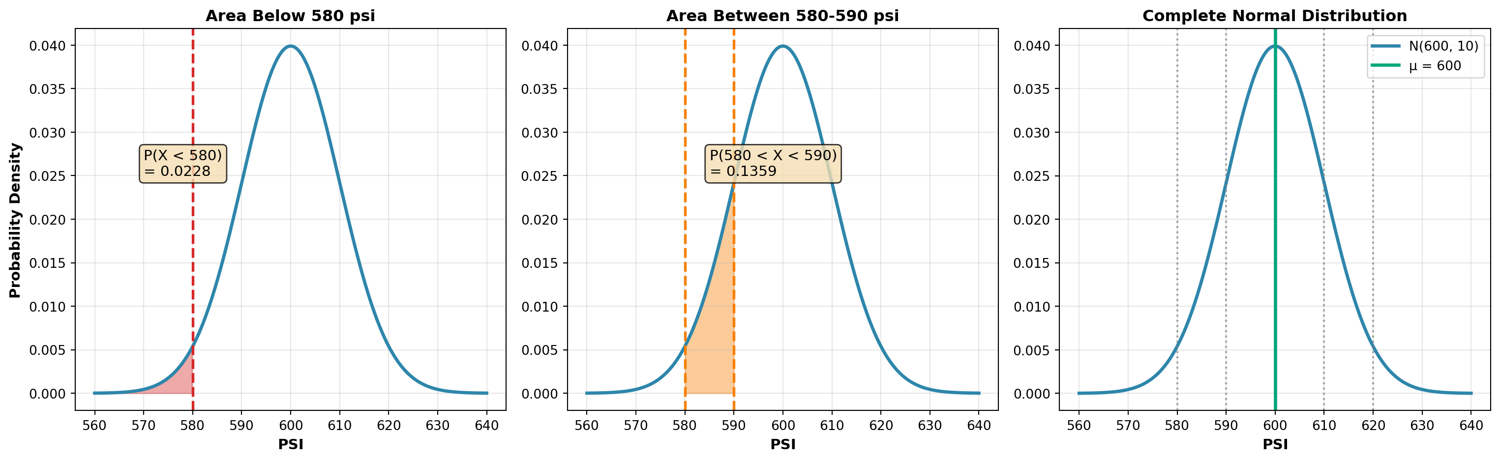
Complete Probability Calculations:
Continuing this process for all intervals:
| PSI Range | Observed (O_i) | Probability (p_i) | Expected (E_i) |
|---|---|---|---|
| Below 580 | 20 | 0.0228 | 22.8 |
| 580 to < 590 | 142 | 0.1359 | 135.9 |
| 590 to < 600 | 310 | 0.3413 | 341.3 |
| 600 to < 610 | 370 | 0.3413 | 341.3 |
| 610 to < 620 | 128 | 0.1359 | 135.9 |
| 620 and above | 30 | 0.0228 | 22.8 |
| Total | 1000 | 1.0000 | 1000.0 |
NoteSymmetric Distribution
Note that for a normal distribution centered at 600, the probabilities (and expected frequencies) are symmetric around the mean. The tails have equal probabilities (0.0228 each).
Calculating Chi-square:
Using \alpha = 0.05, with K = 6 classes and m = 0 (mean and std dev are given, not estimated):
- Degrees of freedom: df = K - m - 1 = 6 - 0 - 1 = 5
- Critical value: \chi^2_{0.05, 5} = 11.07
\begin{aligned} \chi^2 &= \frac{(20-22.8)^2}{22.8} + \frac{(142-135.9)^2}{135.9} + \frac{(310-341.3)^2}{341.3} \\[8pt] &\quad + \frac{(370-341.3)^2}{341.3} + \frac{(128-135.9)^2}{135.9} + \frac{(30-22.8)^2}{22.8} \\[10pt] &= 0.34 + 0.27 + 2.87 + 2.41 + 0.46 + 2.28 \\[10pt] &= 8.63 \end{aligned}
Decision Rule:
- Do not reject H_0 if \chi^2 \leq 11.07
- Reject H_0 if \chi^2 > 11.07
Code
import numpy as np
import matplotlib.pyplot as plt
from scipy.stats import chi2

df = 5
test_statistic = 8.63
critical_value = 11.07
alpha = 0.05

x = np.linspace(0, 20, 500)
y = chi2.pdf(x, df)

fig, ax = plt.subplots(figsize=(12, 7))

# Plot distribution
ax.plot(x, y, linewidth=3, color='#2E86AB', label=f'χ² distribution (df={df})')

# Fill non-rejection region
x_accept = x[x <= critical_value]
y_accept = chi2.pdf(x_accept, df)
ax.fill_between(x_accept, y_accept, alpha=0.2, color='#06A77D',
                 label='Non-rejection region')

# Fill rejection region
x_reject = x[x >= critical_value]
y_reject = chi2.pdf(x_reject, df)
ax.fill_between(x_reject, y_reject, alpha=0.3, color='#D62828',
                 label=f'Rejection region (α = {alpha})')

# Mark critical value
ax.axvline(critical_value, color='#D62828', linestyle='--', linewidth=2.5,
           label=f'Critical value = {critical_value}')

# Mark test statistic
ax.axvline(test_statistic, color='#06A77D', linestyle='-', linewidth=3,
           label=f'Test statistic χ² = {test_statistic}')
ax.plot(test_statistic, chi2.pdf(test_statistic, df), 'o',
        markersize=14, color='#06A77D', zorder=5)

# Add annotation
ax.annotate('DO NOT REJECT H₀', xy=(test_statistic, chi2.pdf(test_statistic, df)),
            xytext=(test_statistic - 3, 0.08),
            fontsize=12, fontweight='bold', color='#06A77D',
            arrowprops=dict(arrowstyle='->', color='#06A77D', lw=2))

ax.set_xlabel('χ² Value', fontsize=13, fontweight='bold')
ax.set_ylabel('Probability Density', fontsize=13, fontweight='bold')
ax.set_title('Chi-square Test for Normality: Scuba Tank Fill Levels',
             fontsize=14, fontweight='bold', pad=20)
ax.legend(fontsize=11, loc='upper right')
ax.grid(True, alpha=0.3, linestyle='--')
ax.set_xlim(0, 20)

plt.tight_layout()
plt.show()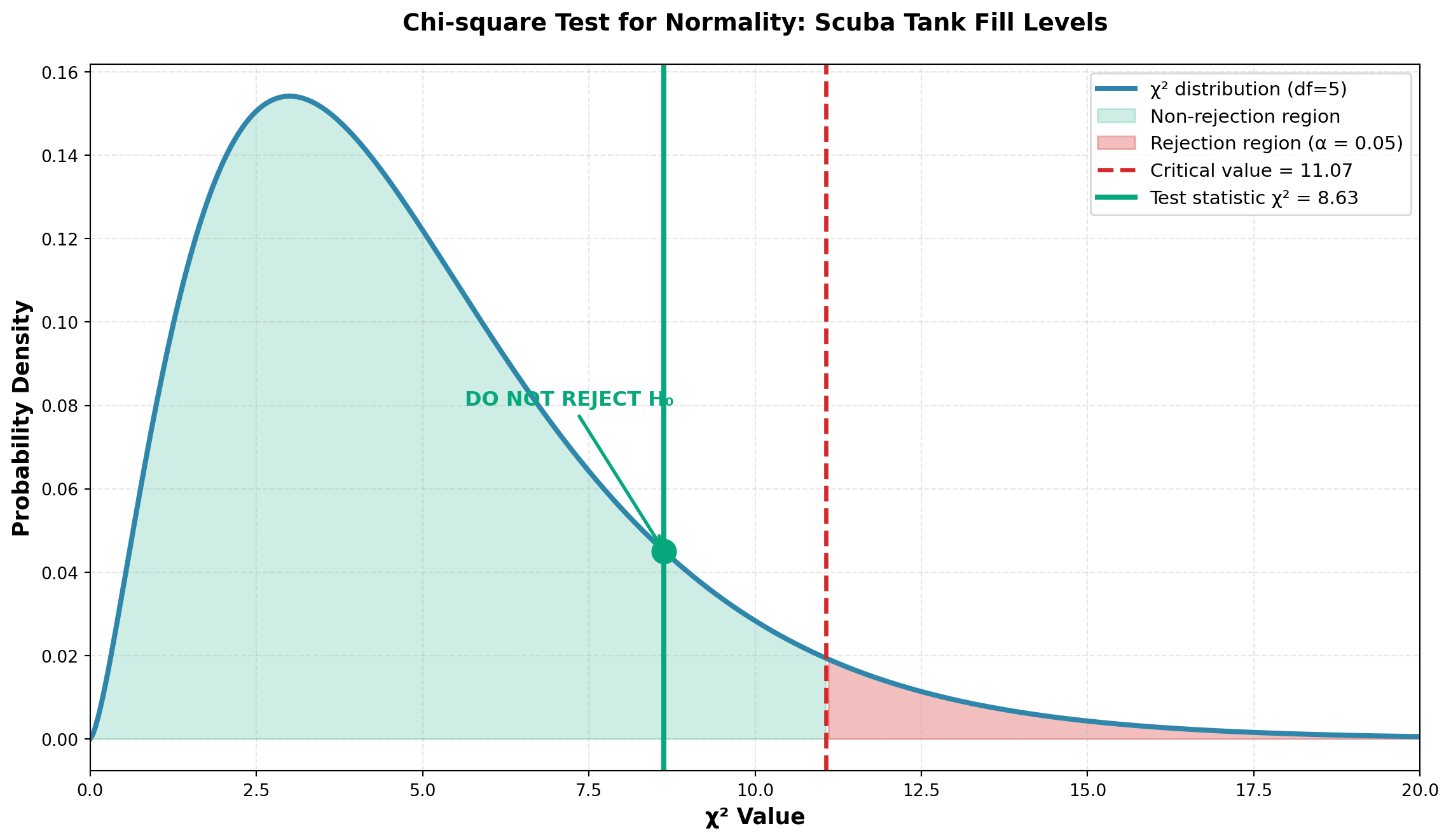
Conclusion:
Since \chi^2 = 8.63 < 11.07 (critical value), we do not reject H_0.
NoteInterpretation
The differences between observed and expected frequencies (assuming normality with \mu = 600 and \sigma = 10) can be attributed to sampling error.
There is insufficient evidence to conclude that fill levels are not normally distributed.
Business implication: The scuba tank filling process appears to meet safety specifications requiring a normal distribution. Production can continue under current quality control standards.
WarningImportant Note About Parameters
If the population mean and standard deviation were unknown and had to be estimated from the sample, then m = 2.
Degrees of freedom would be: df = K - m - 1 = 6 - 2 - 1 = 3
This reduces the degrees of freedom because estimating parameters from the data uses up information.
ImportantCritical Requirement: Minimum Expected Frequency
The chi-square goodness of fit test is reliable only if all expected frequencies E_i \geq 5.
If any E_i < 5:
- Combine that class with adjacent classes until E_i \geq 5 for all categories
- Reduce degrees of freedom correspondingly
Example: If we had sampled only n = 100 tanks instead of 1000:
- First class: E_1 = (100)(0.0228) = 2.28 < 5 ❌
- Last class: E_6 = (100)(0.0228) = 2.28 < 5 ❌
Solution: Combine class 1 with class 2, and class 6 with class 5, reducing from 6 to 4 classes.
15.8 14.6 Contingency Tables: Tests of Independence
So far, all problems have involved one factor of interest. However, chi-square also allows comparison of two attributes to determine whether a relationship exists between them.
Business applications:
- Is there a relationship between customer income level and product preference?
- Is productivity related to type of employee training received?
- Does geographic location affect customer satisfaction ratings?
15.8.1 Example: Dow Chemical Product Effectiveness Study
Scenario: Wilma Keeto, Research Director at Dow Chemical, must determine whether a relationship exists between:
- Attribute A: Effectiveness rating assigned by consumers to a new insecticide
- Attribute B: Location where the product is used (urban vs. rural)
Sample: 100 consumers surveyed:
- 75 from urban areas
- 25 from rural areas
Contingency Table:
| Attribute B: Location | |||
|---|---|---|---|
| Attribute A: Rating | Urban | Rural | Total |
| Above Average | 20 | 11 | 31 |
| Average | 40 | 8 | 48 |
| Below Average | 15 | 6 | 21 |
| Total | 75 | 25 | 100 |
This is a 3 × 2 contingency table (3 rows, 2 columns, 6 cells total).
Hypotheses:
\begin{aligned}
H_0 &: \text{Rating and location are independent} \\
H_A &: \text{Rating and location are NOT independent (they are related)}
\end{aligned}
15.8.2 Logic of Independence Testing
If location has NO impact on ratings (independence), then:
- % of urban residents rating “above average” = % of rural residents rating “above average”
- Both should equal % of all users rating “above average”
From the data: 31 of 100 users (31%) rated the product “above average”
If independence holds:
- 31% of the 75 urban residents should rate it “above average”: (75)(0.31) = 23.3
- 31% of the 25 rural residents should rate it “above average”: (25)(0.31) = 7.75
15.8.3 Calculating All Expected Frequencies
For “Average” rating: 48 of 100 (48%) gave this rating
- Urban expected: (75)(0.48) = 36.0
- Rural expected: (25)(0.48) = 12.0
For “Below Average” rating: 21 of 100 (21%) gave this rating
- Urban expected: (75)(0.21) = 15.75
- Rural expected: (25)(0.21) = 5.25
Complete Table with Expected Frequencies:
| Urban | Rural | Total | |
|---|---|---|---|
| Above Average | O_i = 20 | O_i = 11 | 31 |
| E_i = 23.25 | E_i = 7.75 | ||
| Average | O_i = 40 | O_i = 8 | 48 |
| E_i = 36.00 | E_i = 12.00 | ||
| Below Average | O_i = 15 | O_i = 6 | 21 |
| E_i = 15.75 | E_i = 5.25 | ||
| Total | 75 | 25 | 100 |
15.8.4 Chi-square Test Statistic for Independence
Formula:
\chi^2 = \sum_{i=1}^{rc} \frac{(O_i - E_i)^2}{E_i} {#eq-chi-independence}
Where the sum is over all r \times c cells in the contingency table.
Calculation:
\begin{aligned} \chi^2 &= \frac{(20-23.25)^2}{23.25} + \frac{(11-7.75)^2}{7.75} + \frac{(40-36)^2}{36} \\[8pt] &\quad + \frac{(8-12)^2}{12} + \frac{(15-15.75)^2}{15.75} + \frac{(6-5.25)^2}{5.25} \\[10pt] &= 0.454 + 1.363 + 0.444 + 1.333 + 0.036 + 0.107 \\[10pt] &= 3.74 \end{aligned}
Degrees of Freedom for Contingency Tables:
df = (r - 1)(c - 1)
Where:
- r = number of rows
- c = number of columns
For this problem: df = (3 - 1)(2 - 1) = 2
Test at \alpha = 0.10:
Critical value: \chi^2_{0.10, 2} = 4.605
Decision Rule:
- Do not reject H_0 if \chi^2 \leq 4.605
- Reject H_0 if \chi^2 > 4.605
Code
import numpy as np
import matplotlib.pyplot as plt
from scipy.stats import chi2

df = 2
test_statistic = 3.74
critical_value = 4.605
alpha = 0.10

x = np.linspace(0, 12, 500)
y = chi2.pdf(x, df)

fig, ax = plt.subplots(figsize=(12, 7))

# Plot distribution
ax.plot(x, y, linewidth=3, color='#2E86AB', label=f'χ² distribution (df={df})')

# Fill non-rejection region
x_accept = x[x <= critical_value]
y_accept = chi2.pdf(x_accept, df)
ax.fill_between(x_accept, y_accept, alpha=0.2, color='#06A77D',
                 label='Non-rejection region')

# Fill rejection region
x_reject = x[x >= critical_value]
y_reject = chi2.pdf(x_reject, df)
ax.fill_between(x_reject, y_reject, alpha=0.3, color='#D62828',
                 label=f'Rejection region (α = {alpha})')

# Mark critical value
ax.axvline(critical_value, color='#D62828', linestyle='--', linewidth=2.5,
           label=f'Critical value = {critical_value}')

# Mark test statistic
ax.axvline(test_statistic, color='#06A77D', linestyle='-', linewidth=3,
           label=f'Test statistic χ² = {test_statistic}')
ax.plot(test_statistic, chi2.pdf(test_statistic, df), 'o',
        markersize=14, color='#06A77D', zorder=5)

ax.set_xlabel('χ² Value', fontsize=13, fontweight='bold')
ax.set_ylabel('Probability Density', fontsize=13, fontweight='bold')
ax.set_title('Chi-square Test of Independence: Product Rating vs Location',
             fontsize=14, fontweight='bold', pad=20)
ax.legend(fontsize=11, loc='upper right')
ax.grid(True, alpha=0.3, linestyle='--')
ax.set_xlim(0, 12)

plt.tight_layout()
plt.show()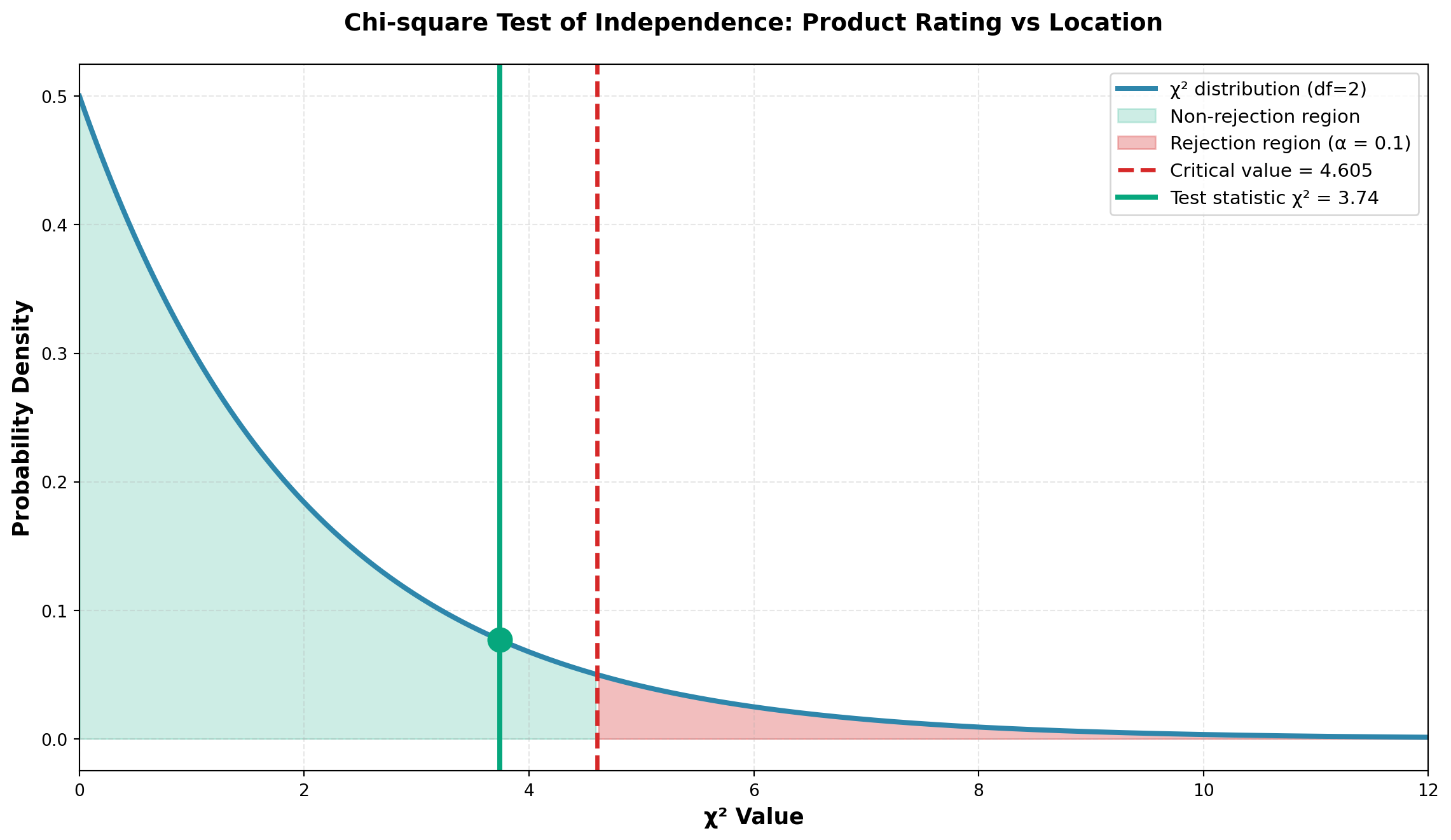
Conclusion:
Since \chi^2 = 3.74 < 4.605 (critical value), we do not reject H_0.
NoteInterpretation
At the 10% significance level, there is insufficient evidence to conclude that product effectiveness ratings and location (urban vs. rural) are related.
The differences between observed and expected frequencies are small enough to be attributed to sampling variation.
Business implication: Dow Chemical can market this insecticide with a unified strategy for both urban and rural areas, as location does not significantly affect perceived effectiveness.
P-value Calculation:
Code
Test statistic: χ² = 3.74
Degrees of freedom: df = 2
P-value = 0.1541

Since p-value (0.1541) > α (0.10), we do not reject H₀
The p-value of 0.155 confirms there is a 15.5% probability of observing differences this large (or larger) if the variables were truly independent.
15.9 14.7 The Sign Test
The sign test is a simple, versatile non-parametric test designed to compare distributions of two populations. It’s particularly useful when parametric assumptions cannot be met.
15.9.1 When to Use the Sign Test
The sign test is appropriate when:
- Paired data is available (before/after, matched pairs)
- The assumption of normality cannot be verified
- You want to test whether one treatment performs better than another
- The data can be reduced to positive (+) and negative (−) signs
TipDefinition: Sign Test
A sign test is designed to test hypotheses comparing the distributions of two populations by examining the signs of differences between paired observations.
Because there are only two possible outcomes (+ or −), and the probability of each remains constant trial after trial, we can use the binomial distribution for the test.
15.9.2 Hypotheses for Sign Tests
Depending on the research question, the sign test can be formulated as:
Two-tailed test:
\begin{aligned}
H_0 &: m = p \\
H_A &: m \neq p
\end{aligned}
Right-tailed test:
\begin{aligned}
H_0 &: m \leq p \\
H_A &: m > p
\end{aligned}
Left-tailed test:
\begin{aligned}
H_0 &: m \geq p \\
H_A &: m < p
\end{aligned}
Where:
- m = number of minus (−) signs
- p = number of plus (+) signs
15.9.3 Example: Promotional Game Effectiveness
Scenario: You’re working as a market analyst measuring the effectiveness of a promotional game for your company’s product.
Study Design:
- Select 12 retail stores
- Record sales for month 1 (before promotion)
- Run promotional game during month 2
- Record sales for month 2 (during promotion)
- Calculate the sign of (Month 1 − Month 2)
Data:
| Store | Before Game | During Game | Difference | Sign |
|---|---|---|---|---|
| 1 | $42 | $40 | +$2 | + |
| 2 | 57 | 60 | −$3 | − |
| 3 | 38 | 38 | $0 | 0 |
| 4 | 49 | 47 | +$2 | + |
| 5 | 63 | 65 | −$2 | − |
| 6 | 36 | 39 | −$3 | − |
| 7 | 48 | 49 | −$1 | − |
| 8 | 58 | 50 | +$8 | + |
| 9 | 47 | 47 | $0 | 0 |
| 10 | 51 | 52 | −$1 | − |
| 11 | 83 | 72 | +$11 | + |
| 12 | 27 | 33 | −$6 | − |
Hypotheses: Test at \alpha = 0.05 whether the promotion increased sales.
If sales increased during month 2 (when promotion was active), subtracting month 2 from month 1 produces minus signs. Therefore, we expect m > p.
\begin{aligned} H_0 &: m \leq p \quad \text{(Promotion had no effect or decreased sales)} \\ H_A &: m > p \quad \text{(Promotion increased sales)} \end{aligned}
Sign Count:
- Minus signs (m): 6
- Plus signs (p): 4
- Zero differences: 2 (ignored)
- Effective sample size: n = 10
ImportantImportant Rule: Zero Differences
Observations with zero difference are eliminated from the analysis and do not count toward the sample size.
Decision Logic:
What would cause us to reject H_0?
Since H_0 states that m \leq p, we reject if:
1. The number of minus signs (m) is significantly large, OR
2. The number of plus signs (p) is significantly small
Probability Calculation:
Using the binomial distribution with n = 10 and \pi = 0.50:
P(m \geq 6 \mid n=10, \pi=0.5) = 1 - P(m \leq 5) = 1 - 0.6230 = 0.3770
Equivalently:
P(p \leq 4 \mid n=10, \pi=0.5) = 0.3770
Code
import numpy as np
import matplotlib.pyplot as plt
from scipy.stats import binom

n = 10
pi = 0.5
k_observed = 6

# Calculate probabilities
k_values = np.arange(0, n+1)
probabilities = binom.pmf(k_values, n, pi)

fig, ax = plt.subplots(figsize=(12, 7))

# Bar plot
bars = ax.bar(k_values, probabilities, color='#2E86AB', alpha=0.7, edgecolor='black')

# Highlight observed value and more extreme
for i, k in enumerate(k_values):
    if k >= k_observed:
        bars[i].set_color('#D62828')
        bars[i].set_alpha(0.8)

# Mark observed value
ax.axvline(k_observed - 0.5, color='#D62828', linestyle='--', linewidth=2.5,
           label=f'Observed: m = {k_observed}')

# Add probability annotation
p_value = 1 - binom.cdf(k_observed - 1, n, pi)
ax.text(8, 0.20, f'P(m ≥ {k_observed}) = {p_value:.4f}\n> α = 0.05',
        fontsize=12, bbox=dict(boxstyle='round', facecolor='wheat', alpha=0.9),
        fontweight='bold')

ax.set_xlabel('Number of Minus Signs (m)', fontsize=13, fontweight='bold')
ax.set_ylabel('Probability', fontsize=13, fontweight='bold')
ax.set_title('Binomial Distribution: Sign Test for Promotional Game (n=10, π=0.5)',
             fontsize=14, fontweight='bold', pad=20)
ax.set_xticks(k_values)
ax.legend(fontsize=11)
ax.grid(True, alpha=0.3, axis='y')

plt.tight_layout()
plt.show()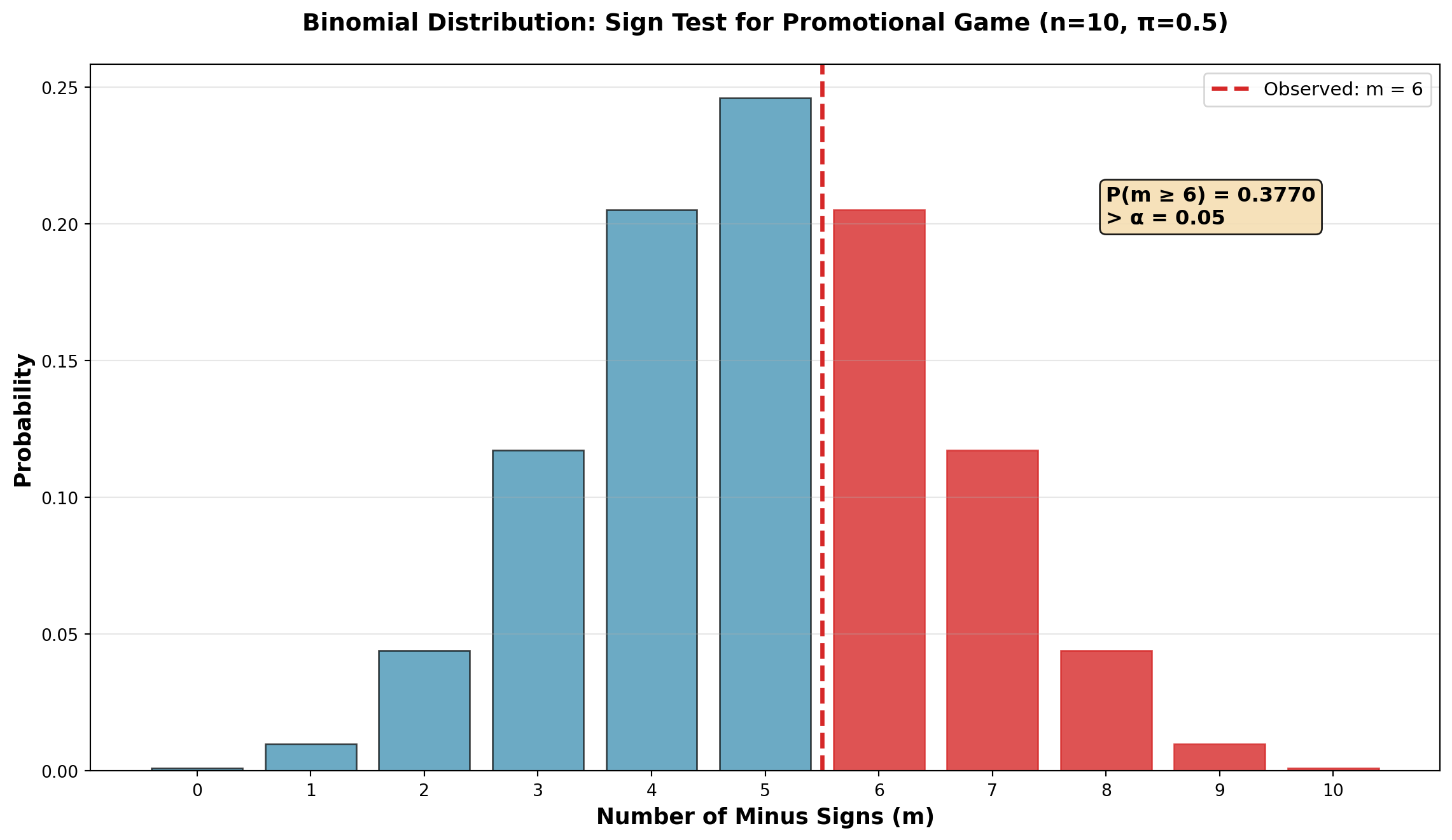
Conclusion:
Since p-value = 0.3770 > \alpha = 0.05, we do not reject H_0.
NoteInterpretation
The probability of obtaining 6 or more minus signs (or 4 or fewer plus signs) when \pi = 0.50 is 37.7% — quite high.
Six minus signs is not an unusually large number. The results can be attributed to sampling variation rather than a genuine promotional effect.
Business implication: The promotional game cannot be considered statistically effective in increasing sales at the 5% significance level. Management should reconsider the promotion strategy or test it with a larger sample.
15.9.4 Sign Test for Large Samples (n \geq 30)
When the sample size is large (n \geq 30), we can use the normal approximation to the binomial.
Test Statistic:
Z = \frac{k \pm 0.5 - 0.5n}{0.5\sqrt{n}} {#eq-sign-test-large}
Where:
- k = number of appropriate signs (+ or −)
- n = sample size (excluding zeros)
- Use k + 0.5 if k < n/2
- Use k − 0.5 if k > n/2
NoteContinuity Correction
The ±0.5 adjustment is necessary because the binomial distribution represents discrete data, while the normal distribution applies to continuous data. This is called a continuity correction.
Example: Honda tire tread test with n = 36, 8 plus signs, 28 minus signs.
Testing for difference (two-tailed test at \alpha = 0.10):
For plus signs (k = 8 < n/2):
Z = \frac{8 + 0.5 - (0.5)(36)}{0.5\sqrt{36}} = \frac{8.5 - 18}{3} = -3.17
For minus signs (k = 28 > n/2):
Z = \frac{28 - 0.5 - (0.5)(36)}{0.5\sqrt{36}} = \frac{27.5 - 18}{3} = 3.17
Critical value at \alpha = 0.10 (two-tailed): Z_{0.05} = \pm 1.65
Since |Z| = 3.17 > 1.65, reject H_0. There is a significant difference between the two tire tread types.
15.10 14.8 The Runs Test
The runs test is a non-parametric test for randomness in the sampling process. Since randomness is essential for valid statistical inference, this test helps verify that samples were drawn randomly.
TipDefinition: Run
A run is a sequence of one or more identical symbols.
Example sequence: A A B B B A B B A A A B
Runs identified:
- Run 1: AA (2 A’s)
- Run 2: BBB (3 B’s)
- Run 3: A (1 A)
- Run 4: BB (2 B’s)
- Run 5: AAA (3 A’s)
- Run 6: B (1 B)
Total: 6 runs
15.10.1 Detecting Patterns vs. Randomness
Key insight: If randomness is absent, we expect:
- Too few runs → systematic pattern (e.g., MMM FFF MMM)
- Too many runs → alternating pattern (e.g., M F M F M F)
Both indicate non-random selection.
15.10.2 Example: Employee Selection by Gender
Suppose employees are selected for a training program. If selection is independent of gender (M = male, F = female), we expect gender to occur randomly.
Sample selection order: M FFF MMM FF MMM
Analysis:
- Run 1: M (1 male)
- Run 2: FFF (3 females)
- Run 3: MMM (3 males)
- Run 4: FF (2 females)
- Run 5: MMM (3 males)
Total: r = 5 runs
Counts: n_1 = 7 males, n_2 = 5 females
Hypotheses:
\begin{aligned}
H_0 &: \text{Randomness exists in the sample} \\
H_A &: \text{Randomness does NOT exist in the sample}
\end{aligned}
Critical Values (from runs table at \alpha = 0.05):
For n_1 = 7 and n_2 = 5:
- Lower critical value: r_L = 3 (too few runs)
- Upper critical value: r_U = 11 (too many runs)
Decision Rule:
- Do not reject H_0 if 3 < r < 11
- Reject H_0 if r \leq 3 or r \geq 11
Since r = 5 falls within the acceptable range, we do not reject H_0. The selection appears random at the 5% significance level.
Code
import numpy as np
import matplotlib.pyplot as plt

fig, axes = plt.subplots(3, 1, figsize=(14, 10))

# Pattern 1: Too few runs (systematic)
pattern1 = ['M']*3 + ['F']*6 + ['M']*3
colors1 = ['#2E86AB' if x == 'M' else '#D62828' for x in pattern1]
axes[0].bar(range(len(pattern1)), [1]*len(pattern1), color=colors1, edgecolor='black', linewidth=2)
axes[0].set_title('Pattern 1: Too FEW Runs (r=3) → Systematic, NON-random',
                  fontsize=13, fontweight='bold', color='#D62828')
axes[0].set_ylabel('Gender', fontsize=11, fontweight='bold')
axes[0].set_yticks([])
axes[0].set_xticks(range(len(pattern1)))
axes[0].set_xticklabels(pattern1, fontsize=10)
axes[0].text(0.5, 0.5, 'Run 1\n(M)', ha='center', va='center', fontweight='bold', fontsize=9)
axes[0].text(5, 0.5, 'Run 2\n(F)', ha='center', va='center', fontweight='bold', fontsize=9)
axes[0].text(10, 0.5, 'Run 3\n(M)', ha='center', va='center', fontweight='bold', fontsize=9)
axes[0].grid(False)

# Pattern 2: Too many runs (alternating)
pattern2 = ['M', 'F'] * 6
colors2 = ['#2E86AB' if x == 'M' else '#D62828' for x in pattern2]
axes[1].bar(range(len(pattern2)), [1]*len(pattern2), color=colors2, edgecolor='black', linewidth=2)
axes[1].set_title('Pattern 2: Too MANY Runs (r=12) → Alternating, NON-random',
                  fontsize=13, fontweight='bold', color='#D62828')
axes[1].set_ylabel('Gender', fontsize=11, fontweight='bold')
axes[1].set_yticks([])
axes[1].set_xticks(range(len(pattern2)))
axes[1].set_xticklabels(pattern2, fontsize=10)
axes[1].grid(False)

# Pattern 3: Appropriate runs (random-looking)
pattern3 = ['M', 'F', 'F', 'F', 'M', 'M', 'M', 'F', 'F', 'M', 'M', 'M']
colors3 = ['#2E86AB' if x == 'M' else '#D62828' for x in pattern3]
axes[2].bar(range(len(pattern3)), [1]*len(pattern3), color=colors3, edgecolor='black', linewidth=2)
axes[2].set_title('Pattern 3: Moderate Runs (r=5) → Appears RANDOM ✓',
                  fontsize=13, fontweight='bold', color='#06A77D')
axes[2].set_ylabel('Gender', fontsize=11, fontweight='bold')
axes[2].set_yticks([])
axes[2].set_xticks(range(len(pattern3)))
axes[2].set_xticklabels(pattern3, fontsize=10)
axes[2].set_xlabel('Selection Order', fontsize=11, fontweight='bold')
axes[2].grid(False)

# Add run markers for pattern 3
run_positions = [0.5, 3, 6, 8, 10.5]
run_labels = ['R1', 'R2', 'R3', 'R4', 'R5']
for pos, label in zip(run_positions, run_labels):
    axes[2].text(pos, 0.5, label, ha='center', va='center',
                 fontweight='bold', fontsize=9, color='white',
                 bbox=dict(boxstyle='circle', facecolor='black', alpha=0.7))

plt.tight_layout()
plt.show()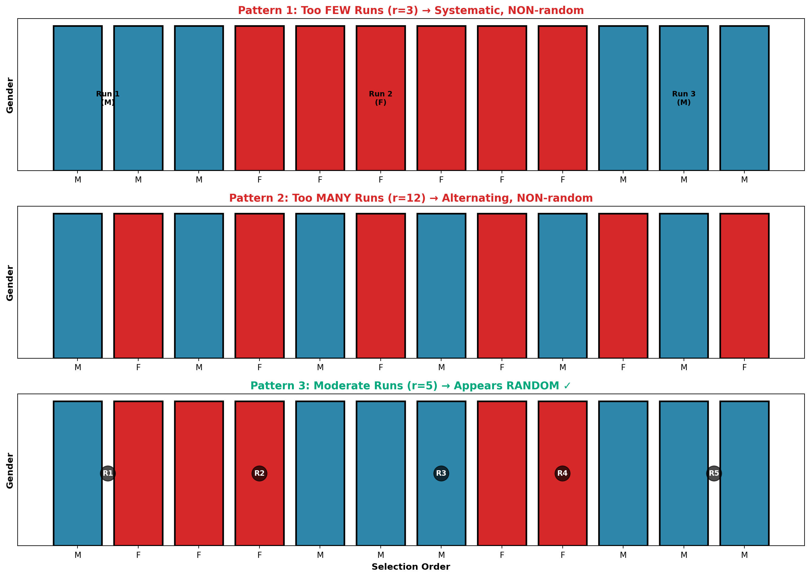
15.10.3 Runs Test for Large Samples (n_1, n_2 > 20)
When both n_1 and n_2 exceed 20, the sampling distribution of r approximates normality.
Mean:
\mu_r = \frac{2n_1 n_2}{n_1 + n_2} + 1
{#eq-runs-mean}
Standard Deviation:
\sigma_r = \sqrt{\frac{2n_1 n_2(2n_1 n_2 - n_1 - n_2)}{(n_1 + n_2)^2(n_1 + n_2 - 1)}}
{#eq-runs-sd}
Test Statistic:
Z = \frac{r - \mu_r}{\sigma_r}
{#eq-runs-z}
Example: Sales presentation to 52 potential buyers resulted in:
- 27 sales
- 25 non-sales
- 18 runs
Test at \alpha = 0.01 (two-tailed):
\mu_r = \frac{2(27)(25)}{27 + 25} + 1 = \frac{1350}{52} + 1 = 26.96
\sigma_r = \sqrt{\frac{2(27)(25)[2(27)(25) - 27 - 25]}{(52)^2(51)}} = \sqrt{\frac{1350 \times 1298}{2704 \times 51}} = 3.56
Z = \frac{18 - 26.96}{3.56} = \frac{-8.96}{3.56} = -2.52
Critical value: Z_{0.005} = \pm 2.58
Since |Z| = 2.52 < 2.58, we do not reject H_0. The sample appears random at the 1% significance level.
Code
import numpy as np
import matplotlib.pyplot as plt
from scipy.stats import norm

mu_r = 26.96
sigma_r = 3.56
r_observed = 18
z_stat = -2.52
z_critical = 2.58

x = np.linspace(mu_r - 4*sigma_r, mu_r + 4*sigma_r, 500)
y = norm.pdf(x, mu_r, sigma_r)

fig, ax = plt.subplots(figsize=(12, 7))

# Plot distribution
ax.plot(x, y, linewidth=3, color='#2E86AB', label='Sampling distribution of r')

# Fill non-rejection region
x_accept = x[(x >= mu_r - z_critical*sigma_r) & (x <= mu_r + z_critical*sigma_r)]
y_accept = norm.pdf(x_accept, mu_r, sigma_r)
ax.fill_between(x_accept, y_accept, alpha=0.2, color='#06A77D',
                 label='Non-rejection region')

# Fill rejection regions
x_reject_left = x[x <= mu_r - z_critical*sigma_r]
y_reject_left = norm.pdf(x_reject_left, mu_r, sigma_r)
ax.fill_between(x_reject_left, y_reject_left, alpha=0.3, color='#D62828')

x_reject_right = x[x >= mu_r + z_critical*sigma_r]
y_reject_right = norm.pdf(x_reject_right, mu_r, sigma_r)
ax.fill_between(x_reject_right, y_reject_right, alpha=0.3, color='#D62828',
                 label='Rejection regions (α = 0.01)')

# Mark critical values
ax.axvline(mu_r - z_critical*sigma_r, color='#D62828', linestyle='--', linewidth=2)
ax.axvline(mu_r + z_critical*sigma_r, color='#D62828', linestyle='--', linewidth=2)

# Mark observed value
ax.axvline(r_observed, color='#F77F00', linestyle='-', linewidth=3,
           label=f'Observed r = {r_observed}, Z = {z_stat}')
ax.plot(r_observed, norm.pdf(r_observed, mu_r, sigma_r), 'o',
        markersize=14, color='#F77F00', zorder=5)

# Mark mean
ax.axvline(mu_r, color='black', linestyle=':', linewidth=2, alpha=0.7,
           label=f'μᵣ = {mu_r:.2f}')

ax.set_xlabel('Number of Runs (r)', fontsize=13, fontweight='bold')
ax.set_ylabel('Probability Density', fontsize=13, fontweight='bold')
ax.set_title('Runs Test: Testing Randomness in Sales Sequence (n₁=27, n₂=25)',
             fontsize=14, fontweight='bold', pad=20)
ax.legend(fontsize=10, loc='upper left')
ax.grid(True, alpha=0.3, linestyle='--')

plt.tight_layout()
plt.show()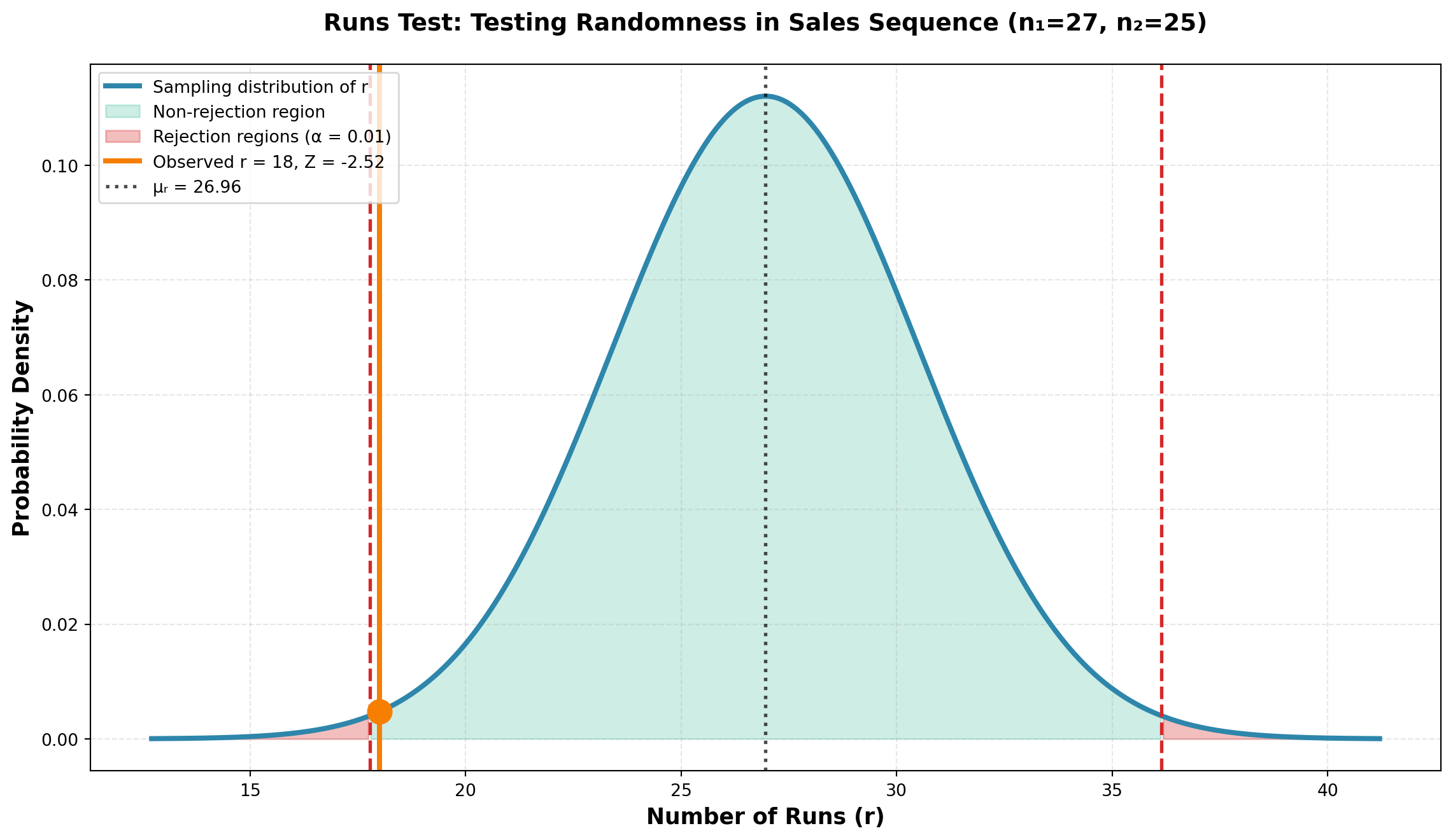
15.11 14.9 Mann-Whitney U Test
The Mann-Whitney U test (also called the Wilcoxon rank-sum test) is the non-parametric counterpart to the independent samples t-test. It tests equality of two population distributions without requiring normality assumptions.
TipDefinition: Mann-Whitney U Test
The Mann-Whitney U test tests the equality of two population distributions based on independent random samples from continuous variables.
Key features:
- No normality assumption required
- Tests equality of medians (or means if populations are symmetric)
- Based on ranks rather than actual values
- Alternative to independent samples t-test
15.11.1 Test Procedure
Steps:
1. Combine all observations from both samples
2. Rank all observations from lowest to highest
3. Sum the ranks for each sample separately
4. Calculate the U statistic for each sample
5. Compare to critical values or use normal approximation
15.11.2 Example: Ceramic Cooling Times
A pottery factory wants to compare cooling times for clay pieces after “firing” in the kiln using two different methods.
Data:
- Method 1: 12 pieces fired
- Method 2: 10 pieces fired
- Measurement: Minutes to cool
| Method 1 | 27 | 31 | 28 | 29 | 39 | 40 | 35 | 33 | 32 | 36 | 37 | 43 |
|---|---|---|---|---|---|---|---|---|---|---|---|---|
| Method 2 | 34 | 24 | 38 | 28 | 30 | 34 | 37 | 42 | 41 | 44 |
Ranking Process:
| Method 1 | Rank | Method 2 | Rank |
|---|---|---|---|
| — | — | 24 | 1 |
| 27 | 2 | — | — |
| 28 | 3.5 | 28 | 3.5 |
| 29 | 5 | — | — |
| — | — | 30 | 6 |
| 31 | 7 | — | — |
| 32 | 8 | — | — |
| 33 | 9 | — | — |
| — | — | 34 | 10.5 |
| — | — | 34 | 10.5 |
| 35 | 12 | — | — |
| 36 | 13 | — | — |
| 37 | 14.5 | 37 | 14.5 |
| — | — | 38 | 16 |
| 39 | 17 | — | — |
| 40 | 18 | — | — |
| — | — | 41 | 19 |
| — | — | 42 | 20 |
| 43 | 21 | — | — |
| — | — | 44 | 22 |
| Sum | \sum R_1 = 130 | Sum | \sum R_2 = 123 |
NoteHandling Tied Values
When values are tied, assign the average rank. For example, both 28’s occupy ranks 3 and 4, so each receives rank (3+4)/2 = 3.5.
Calculate U Statistics:
U_1 = n_1 n_2 + \frac{n_1(n_1 + 1)}{2} - \sum R_1 {#eq-mann-whitney-u1}
U_2 = n_1 n_2 + \frac{n_2(n_2 + 1)}{2} - \sum R_2 {#eq-mann-whitney-u2}
U_1 = (12)(10) + \frac{12(13)}{2} - 130 = 120 + 78 - 130 = 68
U_2 = (12)(10) + \frac{10(11)}{2} - 123 = 120 + 55 - 123 = 52
Check: U_1 + U_2 = 68 + 52 = 120 = n_1 n_2 ✓
15.11.3 Normal Approximation (when n_1, n_2 \geq 10)
Mean:
\mu_U = \frac{n_1 n_2}{2} = \frac{(12)(10)}{2} = 60
Standard Deviation:
\sigma_U = \sqrt{\frac{n_1 n_2(n_1 + n_2 + 1)}{12}} = \sqrt{\frac{(12)(10)(23)}{12}} = \sqrt{230} = 15.17
Test Statistic:
Z = \frac{U_i - \mu_U}{\sigma_U}
{#eq-mann-whitney-z}
15.11.4 Two-Tailed Test
Hypotheses:
\begin{aligned}
H_0 &: \mu_1 = \mu_2 \quad \text{(Cooling times are equal)} \\
H_A &: \mu_1 \neq \mu_2 \quad \text{(Cooling times differ)}
\end{aligned}
For a two-tailed test, use either U_1 or U_2. Using U_2 = 52:
Z = \frac{52 - 60}{15.17} = \frac{-8}{15.17} = -0.53
At \alpha = 0.10, critical value: Z_{0.05} = \pm 1.65
Decision: Since |Z| = 0.53 < 1.65, do not reject H_0.
Code
import numpy as np
import matplotlib.pyplot as plt
from scipy.stats import norm

mu_u = 60
sigma_u = 15.17
z_stat = -0.53
z_critical = 1.65

x = np.linspace(mu_u - 4*sigma_u, mu_u + 4*sigma_u, 500)
y = norm.pdf(x, mu_u, sigma_u)

fig, ax = plt.subplots(figsize=(12, 7))

# Plot distribution
ax.plot(x, y, linewidth=3, color='#2E86AB', label='Sampling distribution of U')

# Fill non-rejection region
x_accept = x[(x >= mu_u - z_critical*sigma_u) & (x <= mu_u + z_critical*sigma_u)]
y_accept = norm.pdf(x_accept, mu_u, sigma_u)
ax.fill_between(x_accept, y_accept, alpha=0.2, color='#06A77D',
                 label='Non-rejection region')

# Fill rejection regions
x_reject_left = x[x <= mu_u - z_critical*sigma_u]
y_reject_left = norm.pdf(x_reject_left, mu_u, sigma_u)
ax.fill_between(x_reject_left, y_reject_left, alpha=0.3, color='#D62828')

x_reject_right = x[x >= mu_u + z_critical*sigma_u]
y_reject_right = norm.pdf(x_reject_right, mu_u, sigma_u)
ax.fill_between(x_reject_right, y_reject_right, alpha=0.3, color='#D62828',
                 label='Rejection regions (α = 0.10)')

# Mark critical values
ax.axvline(mu_u - z_critical*sigma_u, color='#D62828', linestyle='--',
           linewidth=2, label=f'Critical values: Z = ±{z_critical}')
ax.axvline(mu_u + z_critical*sigma_u, color='#D62828', linestyle='--', linewidth=2)

# Mark observed U2
u_observed = 52
ax.axvline(u_observed, color='#06A77D', linestyle='-', linewidth=3,
           label=f'Observed U₂ = {u_observed}, Z = {z_stat}')
ax.plot(u_observed, norm.pdf(u_observed, mu_u, sigma_u), 'o',
        markersize=14, color='#06A77D', zorder=5)

# Mark mean
ax.axvline(mu_u, color='black', linestyle=':', linewidth=2, alpha=0.7,
           label=f'μᵤ = {mu_u}')

ax.set_xlabel('U Statistic Value', fontsize=13, fontweight='bold')
ax.set_ylabel('Probability Density', fontsize=13, fontweight='bold')
ax.set_title('Mann-Whitney U Test: Ceramic Cooling Times (Two-Tailed)',
             fontsize=14, fontweight='bold', pad=20)
ax.legend(fontsize=10, loc='upper left')
ax.grid(True, alpha=0.3, linestyle='--')

plt.tight_layout()
plt.show()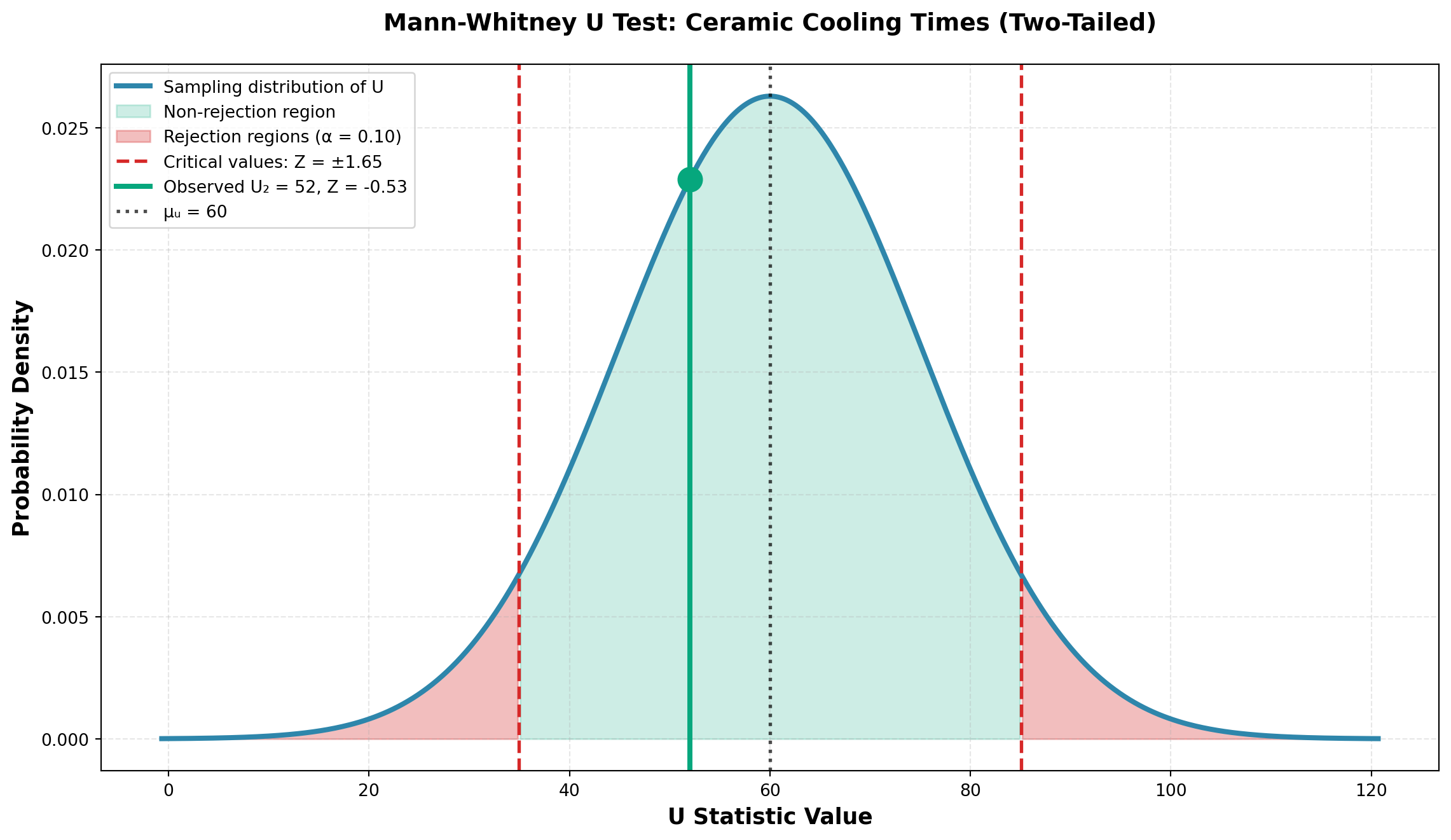
Conclusion:
At the 10% significance level, there is insufficient evidence to conclude that cooling times differ between the two methods.
NoteInterpretation
The Mann-Whitney U test reveals no significant difference in cooling times. The pottery factory can use either method without concern about differential cooling times affecting production schedules.
Business advantage: This flexibility allows the factory to choose methods based on other factors like energy cost, kiln capacity, or production workflow.
15.12 14.10 Spearman Rank Correlation
In many business situations, we need to measure the relationship between two variables when the assumptions required for the Pearson correlation coefficient cannot be met. The Spearman rank correlation coefficient provides a non-parametric alternative that requires only ordinal-level data (rankings) rather than interval or ratio data with a normal distribution.
NoteWhen to Use Spearman Rank Correlation
Use the Spearman rank correlation coefficient when:
- Variables are measured on an ordinal scale (rankings)
- The relationship may not be linear
- Data contains outliers that would distort Pearson correlation
- Sample sizes are small
- Normality assumptions cannot be met
The Spearman rank correlation coefficient, denoted as r_S, measures the strength and direction of association between two ranked variables. Like the Pearson correlation coefficient, r_S ranges from -1 to +1, where:
- r_S = +1 indicates perfect positive association
- r_S = -1 indicates perfect negative association
- r_S = 0 indicates no association
15.12.1 Computing the Spearman Rank Correlation Coefficient
The formula for calculating the Spearman rank correlation coefficient is:
r_S = 1 - \frac{6\sum d_i^2}{n(n^2-1)} \tag{15.2}
where:
- d_i = difference between the ranks for each observation
- n = sample size (number of paired observations)
15.12.2 Example: Amco Tech Employee Performance
Amco Tech, a technology services company, wants to determine whether performance on a written examination is related to actual job performance. The personnel director selects seven technicians and records both their test scores and their performance rankings by supervisors. The data are shown in Table 14.9.
| Technician | Test Score | Test Rank (X) | Performance Rank (Y) | d_i = X - Y | d_i^2 |
|---|---|---|---|---|---|
| J. Smith | 82 | 3 | 4 | -1 | 1 |
| A. Jones | 73 | 5 | 7 | -2 | 4 |
| D. Boone | 60 | 7 | 6 | 1 | 1 |
| M. Lewis | 80 | 4 | 3 | 1 | 1 |
| G. Clark | 67 | 6 | 5 | 1 | 1 |
| A. Lincoln | 94 | 1 | 1 | 0 | 0 |
| G. Washington | 89 | 2 | 2 | 0 | 0 |
| Total: | 8 |
The test scores are ranked from highest to lowest (highest score receives rank 1). Performance is also ranked from best to worst. The differences between rankings are calculated and squared.
Using Equation 15.2:
\begin{aligned} r_S &= 1 - \frac{6\sum d_i^2}{n(n^2-1)} \\[10pt] &= 1 - \frac{6(8)}{7(7^2-1)} \\[10pt] &= 1 - \frac{48}{7(48)} \\[10pt] &= 1 - \frac{48}{336} \\[10pt] &= 1 - 0.143 \\[10pt] &= 0.857 \end{aligned}
TipInterpretation
The sample Spearman correlation coefficient of r_S = 0.857 suggests a strong positive relationship between test scores and job performance rankings. Technicians who score higher on the written examination tend to receive better performance evaluations from their supervisors.
15.12.3 Hypothesis Testing for Spearman Correlation
Often we want to test whether the population rank correlation coefficient, \rho_S, is significantly different from zero. Even when the sample suggests a relationship, we must determine if this could have occurred by chance.
Hypotheses:
\begin{aligned} H_0&: \rho_S = 0 \quad \text{(No relationship between variables)} \\ H_a&: \rho_S \neq 0 \quad \text{(A relationship exists between variables)} \end{aligned}
15.12.3.1 Small Samples (n < 30)
For small samples, the distribution of r_S is not normal, and the t-test is not appropriate. Instead, we use critical values from the Spearman correlation table (Appendix Table N in most statistics textbooks).
For the Amco Tech example with n = 7 at \alpha = 0.10 (two-tailed test):
- Critical values: r_{S,critical} = \pm 0.6786
Decision Rule:
Do not reject H_0 if -0.6786 \leq r_S \leq 0.6786
Reject H_0 if r_S < -0.6786 or r_S > 0.6786
Since our calculated r_S = 0.857 > 0.6786, we reject the null hypothesis at the 10% significance level.
Code
import numpy as np
import matplotlib.pyplot as plt

# Parameters
alpha = 0.10
critical_value = 0.6786
observed_rs = 0.857

# Create x-axis for r_S values
rs_values = np.linspace(-1, 1, 1000)

# Create a "pseudo-distribution" for visualization
# Since exact distribution is complex for small n, we'll show regions
fig, ax = plt.subplots(figsize=(10, 6))

# Rejection regions (red)
ax.axvspan(-1, -critical_value, alpha=0.3, color='red', label='Rejection Region (α/2)')
ax.axvspan(critical_value, 1, alpha=0.3, color='red')

# Non-rejection region (green)
ax.axvspan(-critical_value, critical_value, alpha=0.3, color='green',
           label='Non-Rejection Region')

# Critical value lines
ax.axvline(x=-critical_value, color='red', linestyle='--', linewidth=2,
           label=f'Critical values: ±{critical_value}')
ax.axvline(x=critical_value, color='red', linestyle='--', linewidth=2)

# Observed value
ax.axvline(x=observed_rs, color='blue', linestyle='-', linewidth=3,
           label=f'Observed r_S = {observed_rs}')

# Add annotations
ax.annotate(f'r_S = {observed_rs}', xy=(observed_rs, 0.5),
            xytext=(observed_rs - 0.15, 0.6),
            fontsize=12, fontweight='bold',
            arrowprops=dict(arrowstyle='->', color='blue', lw=2))

ax.annotate('REJECT H₀', xy=(0.85, 0.3), fontsize=11,
            color='darkred', fontweight='bold')
ax.annotate('REJECT H₀', xy=(-0.9, 0.3), fontsize=11,
            color='darkred', fontweight='bold')
ax.annotate('Do Not Reject H₀', xy=(-0.15, 0.3), fontsize=11,
            color='darkgreen', fontweight='bold')

# Labels and formatting
ax.set_xlabel('Spearman Rank Correlation Coefficient (r_S)', fontsize=12)
ax.set_ylabel('Decision Regions', fontsize=12)
ax.set_title('Spearman Rank Correlation Test: Amco Tech (n=7, α=0.10)',
             fontsize=14, fontweight='bold')
ax.set_ylim(0, 1)
ax.set_xlim(-1, 1)
ax.set_yticks([])
ax.legend(loc='upper left', fontsize=10)
ax.grid(True, alpha=0.3)

plt.tight_layout()
plt.show()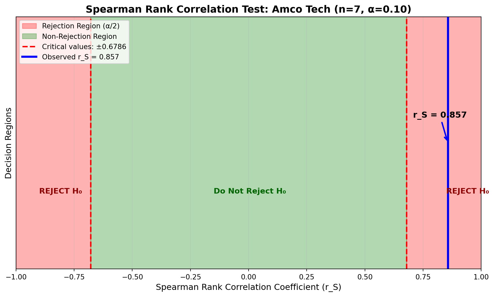
ImportantBusiness Conclusion
At the 10% significance level, there is statistically significant evidence of a positive relationship between written test performance and actual job performance. Amco Tech can use the written examination as a valid screening tool for predicting employee job performance.
15.12.3.2 Large Samples (n \geq 30)
When the sample size is 30 or larger, the distribution of r_S approximates a normal distribution with:
- Mean: \mu_{r_S} = 0
- Standard deviation: \sigma_{r_S} = \frac{1}{\sqrt{n-1}}
The test statistic becomes:
Z = \frac{r_S - 0}{1/\sqrt{n-1}} = r_S\sqrt{n-1} \tag{15.3}
This Z-value can be compared to critical values from the standard normal distribution.
15.12.4 Example: Amco Tech Hard Drive Testing (Large Sample)
Amco Tech is considering whether to market a hard drive for desktop computers. An experiment with 32 randomly selected hard drives examines the relationship between testing hours (before sale) and failure rates (number of times the drive fails to complete running a computer program).
The quality control manager expects that failure rates should decrease as testing hours increase. The data for all 32 drives, including testing hours, failure counts, and their respective rankings, are shown in Table 14.10.
| Drive | Hours | Rank (X) | Failures | Rank (Y) | d_i = X - Y | d_i^2 |
|---|---|---|---|---|---|---|
| 1 | 100 | 1.0 | 2 | 32.0 | -31.0 | 961.00 |
| 2 | 99 | 2.5 | 3 | 30.5 | -28.0 | 784.00 |
| 3 | 99 | 2.5 | 3 | 30.5 | -28.0 | 784.00 |
| 4 | 97 | 4.0 | 4 | 28.5 | -24.5 | 600.25 |
| 5 | 96 | 5.5 | 4 | 28.5 | -23.0 | 529.00 |
| 6 | 96 | 5.5 | 5 | 27.0 | -21.5 | 462.25 |
| 7 | 95 | 7.0 | 8 | 21.5 | -14.5 | 210.25 |
| 8 | 91 | 8.0 | 6 | 25.5 | -17.5 | 306.25 |
| 9 | 89 | 9.0 | 7 | 23.5 | -14.5 | 210.25 |
| 10 | 88 | 10.5 | 10 | 17.5 | -7.0 | 49.00 |
| 11 | 88 | 10.5 | 8 | 21.5 | -11.0 | 121.00 |
| 12 | 80 | 12.0 | 9 | 19.5 | -7.5 | 56.25 |
| 13 | 79 | 13.0 | 9 | 19.5 | -6.5 | 42.25 |
| 14 | 78 | 14.5 | 10 | 17.5 | -3.0 | 9.00 |
| 15 | 78 | 14.5 | 11 | 15.5 | -1.0 | 1.00 |
| 16 | 77 | 16.0 | 7 | 23.5 | -7.5 | 56.25 |
| 17 | 75 | 17.5 | 12 | 13.5 | 4.0 | 16.00 |
| 18 | 75 | 17.5 | 13 | 12.0 | 5.5 | 30.25 |
| 19 | 71 | 19.0 | 11 | 15.5 | 3.5 | 12.25 |
| 20 | 70 | 20.5 | 14 | 11.0 | 9.5 | 90.25 |
| 21 | 70 | 20.5 | 12 | 13.5 | 7.0 | 49.00 |
| 22 | 68 | 22.5 | 6 | 25.5 | -3.0 | 9.00 |
| 23 | 68 | 22.5 | 16 | 7.5 | 15.0 | 225.00 |
| 24 | 65 | 24.0 | 15 | 9.5 | 14.5 | 210.25 |
| 25 | 64 | 25.0 | 15 | 9.5 | 15.5 | 240.25 |
| 26 | 60 | 26.5 | 16 | 7.5 | 19.0 | 361.00 |
| 27 | 60 | 26.5 | 18 | 3.5 | 23.0 | 529.00 |
| 28 | 58 | 28.0 | 19 | 2.0 | 26.0 | 676.00 |
| 29 | 56 | 29.0 | 17 | 5.5 | 23.5 | 552.25 |
| 30 | 55 | 30.5 | 20 | 1.0 | 29.5 | 870.25 |
| 31 | 55 | 30.5 | 18 | 3.5 | 27.0 | 729.00 |
| 32 | 50 | 32.0 | 17 | 5.5 | 26.5 | 702.25 |
| Total: | 10,484.00 |
Note that both variables are ranked from highest to lowest (highest hours receives rank 1, most failures receives rank 1). Tied values are assigned average ranks.
Calculation:
\begin{aligned} r_S &= 1 - \frac{6\sum d_i^2}{n(n^2-1)} \\[10pt] &= 1 - \frac{6(10,484)}{32(32^2-1)} \\[10pt] &= 1 - \frac{62,904}{32(1,023)} \\[10pt] &= 1 - \frac{62,904}{32,736} \\[10pt] &= 1 - 1.922 \\[10pt] &= -0.922 \end{aligned}
Hypothesis Test:
\begin{aligned} H_0&: \rho_S = 0 \quad \text{(No relationship)} \\ H_a&: \rho_S \neq 0 \quad \text{(A relationship exists)} \end{aligned}
At \alpha = 0.01 (two-tailed), the critical Z-values are \pm 2.58.
Using Equation 15.3:
\begin{aligned} Z &= r_S\sqrt{n-1} \\ &= (-0.922)\sqrt{32-1} \\ &= (-0.922)\sqrt{31} \\ &= (-0.922)(5.568) \\ &= -5.14 \end{aligned}
Code
import numpy as np
import matplotlib.pyplot as plt
from scipy.stats import norm

# Parameters
alpha = 0.01
z_critical = 2.58
observed_z = -5.14
n = 32

# Create x-axis
z_values = np.linspace(-6, 6, 1000)
normal_curve = norm.pdf(z_values, 0, 1)

# Create plot
fig, ax = plt.subplots(figsize=(12, 7))

# Plot normal distribution
ax.plot(z_values, normal_curve, 'black', linewidth=2, label='Standard Normal Distribution')

# Fill rejection regions
left_tail = z_values[z_values <= -z_critical]
ax.fill_between(left_tail, norm.pdf(left_tail, 0, 1), alpha=0.3, color='red',
                label=f'Rejection Region (α/2 = {alpha/2})')

right_tail = z_values[z_values >= z_critical]
ax.fill_between(right_tail, norm.pdf(right_tail, 0, 1), alpha=0.3, color='red')

# Fill non-rejection region
middle = z_values[(z_values >= -z_critical) & (z_values <= z_critical)]
ax.fill_between(middle, norm.pdf(middle, 0, 1), alpha=0.3, color='green',
                label='Non-Rejection Region')

# Critical value lines
ax.axvline(x=-z_critical, color='red', linestyle='--', linewidth=2,
           label=f'Critical values: Z = ±{z_critical}')
ax.axvline(x=z_critical, color='red', linestyle='--', linewidth=2)

# Observed Z value
ax.axvline(x=observed_z, color='blue', linestyle='-', linewidth=3,
           label=f'Observed Z = {observed_z}')

# Mean line
ax.axvline(x=0, color='black', linestyle=':', linewidth=1.5, alpha=0.7)

# Annotations
ax.annotate(f'Z = {observed_z}', xy=(observed_z, 0.02),
            xytext=(observed_z + 0.5, 0.08),
            fontsize=12, fontweight='bold', color='blue',
            arrowprops=dict(arrowstyle='->', color='blue', lw=2))

ax.annotate('REJECT H₀', xy=(-4.5, 0.15), fontsize=11,
            color='darkred', fontweight='bold')
ax.annotate('REJECT H₀', xy=(3.5, 0.15), fontsize=11,
            color='darkred', fontweight='bold')

ax.text(0, 0.25, f'r_S = -0.922\nn = 32', ha='center',
        fontsize=11, bbox=dict(boxstyle='round', facecolor='wheat', alpha=0.8))

# Labels and formatting
ax.set_xlabel('Z-value', fontsize=12)
ax.set_ylabel('Probability Density', fontsize=12)
ax.set_title('Large Sample Spearman Rank Correlation Test\nHard Drive Testing Hours vs. Failure Rates',
             fontsize=14, fontweight='bold')
ax.legend(loc='upper right', fontsize=10)
ax.grid(True, alpha=0.3)
ax.set_xlim(-6, 6)

plt.tight_layout()
plt.show()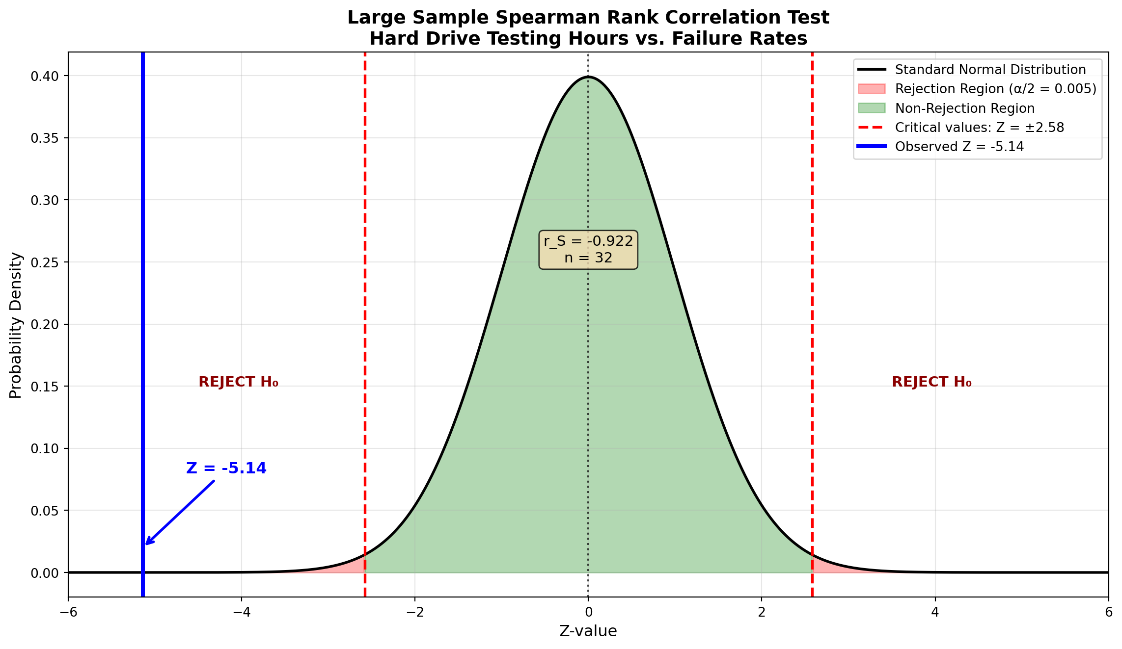
Decision:
Since Z = -5.14 < -2.58, we reject the null hypothesis at the 1% significance level.
ImportantInterpretation and Business Recommendation
The Spearman correlation coefficient of r_S = -0.922 indicates a strong negative relationship between testing hours and failure rates. The more a hard drive is tested before sale, the fewer failures it experiences when running complete programs.
Business Implication: Amco Tech should implement rigorous pre-sale testing procedures to minimize customer-reported failures and warranty claims. The statistical evidence strongly supports increased quality control testing.
15.13 14.11 The Kruskal-Wallis Test
The Mann-Whitney U test serves as the non-parametric alternative to the independent samples t-test for comparing two populations. When we need to compare three or more populations, the Kruskal-Wallis test provides the appropriate non-parametric extension.
NoteKruskal-Wallis Test Overview
The Kruskal-Wallis test is the non-parametric counterpart to one-way ANOVA. While ANOVA requires that all populations being compared are normally distributed, the Kruskal-Wallis test places no such restriction.
Use when:
- Comparing three or more independent groups
- Normality assumptions cannot be met
- Data are ordinal or contain outliers
- Sample sizes are small
15.13.1 Hypotheses
The null hypothesis states that there is no difference in the distributions of the k populations being compared:
\begin{aligned} H_0&: \text{All } k \text{ populations have the same distribution} \\ H_a&: \text{Not all } k \text{ populations have the same distribution} \end{aligned}
15.13.2 Test Procedure
The Kruskal-Wallis test requires that all observations from all samples be ranked together from lowest to highest, similar to the Mann-Whitney U test.
15.13.3 Example: Pox Skin Ointment Payment Times
As the new accounts manager for Pox Skin Ointment, you need to compare the payment times for three major customers who purchase No-Flaw-Face Cream. Several purchases from each customer are randomly selected, and the number of days to settle each account is recorded.
The data are shown in Table 14.11.
| Purchase | Customer 1 | Customer 2 | Customer 3 |
|---|---|---|---|
| 1 | 28 | 26 | 37 |
| 2 | 19 | 20 | 28 |
| 3 | 13 | 11 | 26 |
| 4 | 28 | 14 | 35 |
| 5 | 29 | 22 | 31 |
| 6 | 22 | 21 | — |
| 7 | 21 | — | — |
Note that sample sizes do not need to be equal: n_1 = 7, n_2 = 6, n_3 = 5, with total n = 18.
15.13.4 Ranking the Data
All 18 observations are ranked from lowest to highest. Tied values receive the average of the ranks they would occupy.
| Customer 1 | Customer 2 | Customer 3 | |||
|---|---|---|---|---|---|
| Days | Rank | Days | Rank | Days | Rank |
| — | — | 11 | 1 | — | — |
| 13 | 2 | — | — | — | — |
| — | — | 14 | 3 | — | — |
| 19 | 4 | — | — | — | — |
| — | — | 20 | 5 | — | — |
| 21 | 6.5 | 21 | 6.5 | — | — |
| 22 | 8.5 | 22 | 8.5 | — | — |
| — | — | 26 | 10.5 | 26 | 10.5 |
| 28 | 13 | — | — | 28 | 13 |
| 28 | 13 | — | — | — | — |
| 29 | 15 | — | — | — | — |
| — | — | — | — | 31 | 16 |
| — | — | — | — | 35 | 17 |
| — | — | — | — | 37 | 18 |
| \sum R_1 = 62 | \sum R_2 = 34.5 | \sum R_3 = 74.5 |
Tied Rank Calculations:
- Days = 21: Two occurrences would occupy ranks 6 and 7, so each receives (6+7)/2 = 6.5
- Days = 22: Two occurrences would occupy ranks 8 and 9, so each receives (8+9)/2 = 8.5
- Days = 26: Two occurrences would occupy ranks 10 and 11, so each receives (10+11)/2 = 10.5
- Days = 28: Two occurrences would occupy ranks 12 and 13, so each receives (12+13)/2 = 13
15.13.5 The Kruskal-Wallis Test Statistic
The test statistic K is calculated using:
K = \frac{12}{n(n+1)}\left[\sum_{i=1}^{k} \frac{R_i^2}{n_i}\right] - 3(n+1) \tag{15.4}
where:
- n_i = number of observations in the i-th sample
- n = total number of observations across all samples
- R_i = sum of ranks for the i-th sample
- k = number of samples (groups)
For the Pox example:
\begin{aligned} K &= \frac{12}{n(n+1)}\left[\frac{R_1^2}{n_1} + \frac{R_2^2}{n_2} + \frac{R_3^2}{n_3}\right] - 3(n+1) \\[10pt] &= \frac{12}{18(19)}\left[\frac{(62)^2}{7} + \frac{(34.5)^2}{6} + \frac{(74.5)^2}{5}\right] - 3(19) \\[10pt] &= \frac{12}{342}\left[\frac{3,844}{7} + \frac{1,190.25}{6} + \frac{5,550.25}{5}\right] - 57 \\[10pt] &= 0.0351\left[549.14 + 198.38 + 1,110.05\right] - 57 \\[10pt] &= 0.0351(1,857.57) - 57 \\[10pt] &= 65.20 - 57 \\[10pt] &= 8.18 \end{aligned}
15.13.6 Distribution and Critical Values
The distribution of the K statistic is approximated by the chi-square distribution with df = k - 1 degrees of freedom.
For the Pox example at \alpha = 0.05:
- k = 3 groups (customers)
- df = k - 1 = 3 - 1 = 2
- Critical value: \chi^2_{0.05, 2} = 5.99
Decision Rule:
Do not reject H_0 if K \leq 5.99
Reject H_0 if K > 5.99
Since K = 8.18 > 5.99, we reject the null hypothesis.
Code
import numpy as np
import matplotlib.pyplot as plt
from scipy.stats import chi2

# Parameters
df = 2
alpha = 0.05
chi2_critical = 5.99
observed_K = 8.18

# Create x-axis
x_values = np.linspace(0, 15, 1000)
chi2_curve = chi2.pdf(x_values, df)

# Create plot
fig, ax = plt.subplots(figsize=(12, 7))

# Plot chi-square distribution
ax.plot(x_values, chi2_curve, 'black', linewidth=2,
        label=f'Chi-square Distribution (df = {df})')

# Fill non-rejection region
non_reject = x_values[x_values <= chi2_critical]
ax.fill_between(non_reject, chi2.pdf(non_reject, df), alpha=0.3, color='green',
                label='Non-Rejection Region')

# Fill rejection region
reject = x_values[x_values > chi2_critical]
ax.fill_between(reject, chi2.pdf(reject, df), alpha=0.3, color='red',
                label=f'Rejection Region (α = {alpha})')

# Critical value line
ax.axvline(x=chi2_critical, color='red', linestyle='--', linewidth=2,
           label=f'Critical value: χ² = {chi2_critical}')

# Observed K value
ax.axvline(x=observed_K, color='blue', linestyle='-', linewidth=3,
           label=f'Observed K = {observed_K}')

# Annotations
ax.annotate(f'K = {observed_K}', xy=(observed_K, 0.05),
            xytext=(observed_K + 1.5, 0.15),
            fontsize=12, fontweight='bold', color='blue',
            arrowprops=dict(arrowstyle='->', color='blue', lw=2))

ax.annotate('Do Not\nReject H₀', xy=(2.5, 0.1), fontsize=11,
            color='darkgreen', fontweight='bold', ha='center')
ax.annotate('REJECT H₀', xy=(10, 0.08), fontsize=11,
            color='darkred', fontweight='bold')

ax.text(8, 0.25, f'n₁=7, n₂=6, n₃=5\ndf = k-1 = 2', ha='center',
        fontsize=11, bbox=dict(boxstyle='round', facecolor='wheat', alpha=0.8))

# Labels and formatting
ax.set_xlabel('K Statistic (Chi-square)', fontsize=12)
ax.set_ylabel('Probability Density', fontsize=12)
ax.set_title('Kruskal-Wallis Test: Pox Customer Payment Times\nH₀: All 3 populations have same distribution',
             fontsize=14, fontweight='bold')
ax.legend(loc='upper right', fontsize=10)
ax.grid(True, alpha=0.3)
ax.set_xlim(0, 15)
ax.set_ylim(0, 0.35)

plt.tight_layout()
plt.show()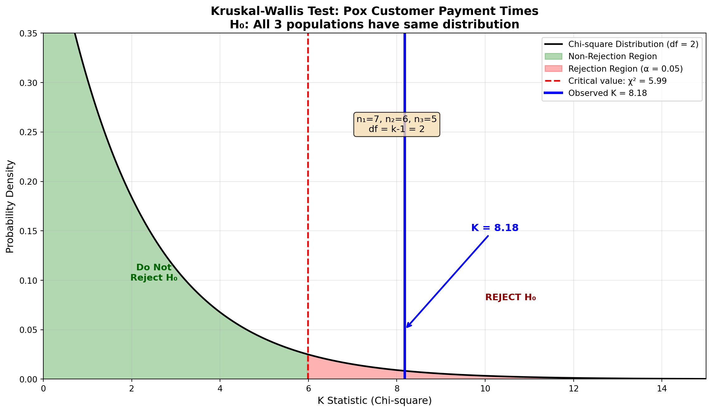
ImportantConclusion
Since K = 8.18 exceeds the critical value of 5.99, we reject the null hypothesis at the 5% significance level. There is statistically significant evidence that the three customers differ in their payment times for Pox shipments.
15.13.7 Post-Hoc Pairwise Comparisons
When we reject the null hypothesis in the Kruskal-Wallis test, the logical next step is to determine which specific pairs of populations differ significantly. This is similar to Tukey’s HSD procedure used after ANOVA.
15.13.7.1 Procedure
- Calculate the average rank for each sample:
\bar{R}_i = \frac{R_i}{n_i}
For the Pox example:
\begin{aligned} \bar{R}_1 &= \frac{62}{7} = 8.86 \\[8pt] \bar{R}_2 &= \frac{34.5}{6} = 5.75 \\[8pt] \bar{R}_3 &= \frac{74.5}{5} = 14.90 \end{aligned}
- Calculate absolute differences between all pairs of average ranks:
\begin{aligned} |\bar{R}_1 - \bar{R}_2| &= |8.86 - 5.75| = 3.11 \\ |\bar{R}_1 - \bar{R}_3| &= |8.86 - 14.90| = 6.04 \\ |\bar{R}_2 - \bar{R}_3| &= |5.75 - 14.90| = 9.15 \end{aligned}
- Calculate the critical difference C_k for each pair:
C_k = \sqrt{\chi^2_{\alpha, k-1} \left[\frac{n(n+1)}{12}\right]\left[\frac{1}{n_i} + \frac{1}{n_j}\right]} \tag{15.5}
where \chi^2_{\alpha, k-1} is the chi-square critical value used in the original test (5.99 in this case).
Comparison 1 vs 2:
\begin{aligned} C_k &= \sqrt{5.99 \left[\frac{18 \times 19}{12}\right]\left[\frac{1}{7} + \frac{1}{6}\right]} \\[8pt] &= \sqrt{5.99 \times 28.5 \times 0.3095} \\[8pt] &= \sqrt{52.83} \\[8pt] &= 7.27 \end{aligned}
Since |\bar{R}_1 - \bar{R}_2| = 3.11 < 7.27, Customer 1 and Customer 2 do not differ significantly.
Comparison 1 vs 3:
\begin{aligned} C_k &= \sqrt{5.99 \left[\frac{18 \times 19}{12}\right]\left[\frac{1}{7} + \frac{1}{5}\right]} \\[8pt] &= \sqrt{5.99 \times 28.5 \times 0.3429} \\[8pt] &= \sqrt{58.53} \\[8pt] &= 7.65 \end{aligned}
Since |\bar{R}_1 - \bar{R}_3| = 6.04 < 7.65, Customer 1 and Customer 3 do not differ significantly.
Comparison 2 vs 3:
\begin{aligned} C_k &= \sqrt{5.99 \left[\frac{18 \times 19}{12}\right]\left[\frac{1}{6} + \frac{1}{5}\right]} \\[8pt] &= \sqrt{5.99 \times 28.5 \times 0.3667} \\[8pt] &= \sqrt{62.60} \\[8pt] &= 7.91 \end{aligned}
Since |\bar{R}_2 - \bar{R}_3| = 9.15 > 7.91, Customer 2 and Customer 3 differ significantly.
15.13.8 Summary Using Common Underlining
Groups that are not significantly different are connected by a common underline:
| \bar{R}_2 | \bar{R}_1 | \bar{R}_3 |
|---|---|---|
| 5.75 | 8.86 | 14.90 |
TipInterpretation
- Customer 2 (average rank 5.75) pays significantly faster than Customer 3 (average rank 14.90)
- Customer 1 (average rank 8.86) is not significantly different from either Customer 2 or Customer 3
- Customers 2 and 1 form one homogeneous group; Customers 1 and 3 overlap in payment behavior
ImportantBusiness Recommendation
Customer 3 takes significantly longer to pay than Customer 2. Pox should:
- Review credit terms with Customer 3
- Consider payment incentives for early settlement
- Adjust inventory allocation based on payment reliability
- Monitor Customer 1’s payment patterns closely as it bridges both groups
15.14 14.12 Comparison of Non-parametric and Parametric Tests
Throughout this chapter, we have explored several non-parametric tests that can be applied when the strict assumptions required by parametric procedures cannot be met. Table 14.12 provides a comprehensive comparison.
| Non-parametric Test | Purpose | Assumption Not Required | Parametric Counterpart |
|---|---|---|---|
| Chi-square Goodness of Fit | Test whether data fits a hypothesized distribution | Specific distribution shape | None (unique) |
| Chi-square Test of Independence | Test relationship between two categorical variables | Normality of variables | Pearson correlation (if continuous) |
| Sign Test | Test location of population distribution using paired data | Normal distribution of differences | Paired t-test |
| Runs Test | Test randomness of sequence | — | None (unique) |
| Mann-Whitney U Test | Compare two independent samples | Normality of populations | Independent samples t-test |
| Spearman Rank Correlation | Test relationship between two ranked/ordinal variables | Normality of both variables | Pearson correlation coefficient |
| Kruskal-Wallis Test | Compare three or more independent samples | Normality of populations | One-way ANOVA (F-test) |
NoteWhen to Choose Non-parametric Tests
Use non-parametric tests when:
- Sample size is small (typically n < 30) and normality cannot be verified
- Data are ordinal (rankings, ratings) rather than interval or ratio scale
- Outliers are present that would distort parametric test results
- Distributions are highly skewed and transformations don’t help
- You want robust results that don’t depend on distribution shape
Trade-offs:
- Advantages: Fewer assumptions, more robust to outliers, work with ordinal data
- Disadvantages: Generally less statistical power than parametric tests when assumptions are met (requires larger sample to detect same effect)
It should now be evident that non-parametric methods provide valuable alternatives when the essential assumptions for parametric procedures cannot be maintained. In the absence of specific conditions such as normally distributed populations, these distribution-free tests often represent the only appropriate course of action.
15.15 Chapter 14 Summary
In this chapter, we explored a comprehensive suite of non-parametric statistical tests that provide powerful alternatives when the strict assumptions of parametric methods cannot be met. These distribution-free procedures are essential tools for modern business analytics.
15.15.1 Key Concepts Covered
15.15.1.1 Chi-square Tests (Sections 14.2–14.6)
- Chi-square Distribution Family
- Right-skewed distributions characterized by degrees of freedom
- Shape becomes less skewed as df increases
- Foundation for goodness-of-fit and independence tests
- Right-skewed distributions characterized by degrees of freedom
- Goodness of Fit Tests
- Test whether observed data fits hypothesized distribution (uniform, specific pattern, normal)
- Test statistic: \chi^2 = \sum \frac{(O_i - E_i)^2}{E_i}
- Degrees of freedom: df = K - m - 1
- Minimum expected frequency requirement: E_i \geq 5
- Test whether observed data fits hypothesized distribution (uniform, specific pattern, normal)
- Contingency Tables and Independence Tests
- Examine relationship between two categorical variables
- Expected frequencies: E_{ij} = \frac{(\text{Row Total})(\text{Column Total})}{n}
- Degrees of freedom: df = (r-1)(c-1)
- Applications: Market segmentation, product preferences, demographic analysis
- Examine relationship between two categorical variables
15.15.1.2 Other Non-parametric Tests (Sections 14.7–14.11)
- Sign Test (Section 14.7)
- Compare paired observations using signs of differences
- Based on binomial distribution
- Small sample: Use binomial probabilities directly
- Large sample (n \geq 30): Z = \frac{k \pm 0.5 - 0.5n}{0.5\sqrt{n}} with continuity correction
- Compare paired observations using signs of differences
- Runs Test (Section 14.8)
- Test randomness of sequences
- Too few runs → systematic pattern
- Too many runs → alternating pattern
- Small sample: Critical values from tables
- Large sample: Normal approximation with \mu_r and \sigma_r
- Test randomness of sequences
- Mann-Whitney U Test (Section 14.9)
- Non-parametric alternative to independent samples t-test
- Based on ranks, not actual values
- Handles tied values through average ranks
- Large sample: Normal approximation Z = \frac{U - \mu_U}{\sigma_U}
- Non-parametric alternative to independent samples t-test
- Spearman Rank Correlation (Section 14.10)
- Measures relationship between ranked variables
- Formula: r_S = 1 - \frac{6\sum d_i^2}{n(n^2-1)}
- Small sample (n < 30): Use critical value tables
- Large sample (n \geq 30): Z = r_S\sqrt{n-1}
- Alternative to Pearson when normality fails
- Measures relationship between ranked variables
- Kruskal-Wallis Test (Section 14.11)
- Non-parametric alternative to one-way ANOVA
- Compares three or more independent groups
- Test statistic: K = \frac{12}{n(n+1)}\left[\sum \frac{R_i^2}{n_i}\right] - 3(n+1)
- Approximated by chi-square with df = k-1
- Post-hoc pairwise comparisons identify specific differences
- Non-parametric alternative to one-way ANOVA
15.15.2 Common Themes Across Non-parametric Methods
NoteFive Unifying Principles
Distribution-Free: No assumption of specific population distribution shape (normal, exponential, etc.)
Rank-Based: Many tests (Mann-Whitney, Kruskal-Wallis, Spearman) use ranks rather than actual values, making them robust to outliers
Flexibility: Work with ordinal, interval, and ratio data; handle small samples effectively
Conservative Power: Generally require larger samples than parametric alternatives to achieve same power when assumptions are met
Practical Utility: Essential when real-world data violates parametric assumptions—which is common in business settings
15.15.3 Strategic Decision Framework
flowchart TD
    Start([What is your<br/>research question?]) --> Question{Data type?}

    Question -->|Categorical| Categorical{How many<br/>variables?}
    Question -->|Ordinal/Ranked| Ranked{How many<br/>groups?}
    Question -->|Sequence/Pattern| Sequence[Runs Test]

    Categorical -->|One variable| Goodness[Chi-square<br/>Goodness of Fit]
    Categorical -->|Two variables| Independence[Chi-square<br/>Independence Test]

    Ranked -->|Paired data| Sign[Sign Test]
    Ranked -->|Two groups| Mann[Mann-Whitney<br/>U Test]
    Ranked -->|Three+ groups| Kruskal[Kruskal-Wallis<br/>Test]
    Ranked -->|Correlation| Spearman[Spearman Rank<br/>Correlation]

    Goodness --> End([Conduct Test])
    Independence --> End
    Sign --> End
    Mann --> End
    Kruskal --> End
    Spearman --> End
    Sequence --> End

    style Start fill:#e1f5ff
    style End fill:#d4edda
    style Goodness fill:#fff3cd
    style Independence fill:#fff3cd
    style Sign fill:#f8d7da
    style Mann fill:#f8d7da
    style Kruskal fill:#f8d7da
    style Spearman fill:#f8d7da
    style Sequence fill:#d1ecf1
15.15.4 Business Applications Summary
Throughout this chapter, we encountered diverse real-world scenarios:
- Mama’s Pizzeria: Market competition analysis (introduction)
- Seven Seas Marina: Boat sales uniform distribution
- John Dillinger Bank: Loan portfolio composition
- Aqua Lung: Scuba tank fill level normality
- Dow Chemical: Product ratings and location independence
- Retail Promotion: Sales effectiveness using sign test
- Employee Selection: Hiring randomness verification
- Ceramic Manufacturing: Cooling time comparison
- Amco Tech: Test scores vs. job performance correlation
- Hard Drive Testing: Quality control and failure rates
- Pox Skin Ointment: Customer payment behavior analysis
These examples demonstrate that non-parametric methods are not merely theoretical—they are practical, essential tools for data-driven business decision-making.
15.15.5 Looking Forward
The techniques in this chapter complement the parametric methods covered earlier in the book. As you encounter real business data, you’ll find that:
- Assumptions matter: Always verify normality, equal variances, and independence before choosing parametric tests
- Flexibility is valuable: Non-parametric tests provide robust alternatives when assumptions fail
- Context drives choice: The nature of your data and research question determines the appropriate test
- Effect size matters: Statistical significance must be paired with practical business significance
TipFinal Thought
Master statisticians and business analysts maintain a toolkit of both parametric and non-parametric methods. The ability to recognize when traditional assumptions are violated—and to confidently apply distribution-free alternatives—is a hallmark of sophisticated quantitative analysis.
As you continue your statistical journey, remember: The goal is not just to run tests, but to extract actionable insights that drive better business decisions.
End of Chapter 14: Chi-square Test and Other Non-parametric Tests