graph TD
    A[Confidence Intervals] --> B[Principle and<br/>Interpretation of<br/>Confidence Intervals]
    A --> C[For Population<br/>Means]
    A --> D[For Population<br/>Proportions]
    A --> E[Controlling the<br/>Width of an<br/>Interval]
    A --> F[Properties of<br/>Good Estimators]
    A --> G[Determination of<br/>Sample Sizes]

    B --> B1[The α value is the<br/>error probability]

    C --> C1[Large Samples]
    C --> C2[Small Samples]

    E --> E1[Change in<br/>Confidence Level]
    E --> E2[Change in<br/>Sample Size]

    F --> F1[Unbiased]
    F --> F2[Efficient]
    F --> F3[Consistent]
    F --> F4[Sufficient]

    G --> G1[To estimate μ]
    G --> G2[To estimate π]

    style A fill:#333,stroke:#000,stroke-width:4px,color:#fff
    style B fill:#fff,stroke:#000,stroke-width:2px
    style C fill:#fff,stroke:#000,stroke-width:2px
    style D fill:#fff,stroke:#000,stroke-width:2px
    style E fill:#fff,stroke:#000,stroke-width:2px
    style F fill:#fff,stroke:#000,stroke-width:2px
    style G fill:#fff,stroke:#000,stroke-width:2px
8 Confidence Intervals
NoteLearning Objectives
After completing this chapter, you will be able to:
- Construct and interpret confidence intervals for population means
- Apply the t-distribution for small sample estimation
- Build confidence intervals for population proportions
- Control interval width through confidence level and sample size adjustments
- Determine appropriate sample sizes for desired precision
- Evaluate estimators using properties of unbiasedness, efficiency, consistency, and sufficiency
- Make business decisions based on interval estimates with specified confidence levels
8.1 Opening Scenario: FBI Statistical Crime Profiling
In 1997, the Federal Bureau of Investigation (FBI) implemented revolutionary procedures to facilitate the capture of persons wanted for serious crimes. A spokesperson from the FBI’s Criminal Statistics Division appeared on CNN’s Larry King Live to discuss procedures that would make city streets safer.
She discussed several statistics the FBI had collected describing motives, techniques, and frequency of crimes that were useful for profiling criminals at large whom the agency wished to capture. Her discussion focused on the agency’s efforts to maintain a large database on criminal statistics that could be used to predict criminal activity and thus anticipate where and when an illegal act might occur.
She mentioned several cases that had been resolved, largely thanks to work done by professional statisticians who provided estimates about recidivism rates of offenders, as well as other activities that provide clues to aid in their arrest. This information proved extremely useful to agents working in the field whose function is to locate those on the FBI’s most wanted list.
The statistical approach to combating crime includes data on a wide variety of crimes, as well as the personal characteristics and habits of offenders. Although the Larry King Live spokesperson did not offer specific details, she stated that data were kept on the number of crimes each law violator commits, the number of days that elapse between crimes, and the number of people killed by law enforcement agencies in arrest attempts.
This scenario illustrates a critical business and public policy application of confidence intervals: making decisions under uncertainty with quantified levels of confidence. Throughout this chapter, we’ll see how managers, researchers, and policy makers use interval estimation to make informed decisions across diverse fields.
8.2 7.1 Introduction to Interval Estimation
You should now be well aware that populations are generally too large to be studied in their entirety. Their size requires that samples be selected, which can later be used to make inferences about the populations. If a retail store manager wants to know the average spending of customers during the previous year, it would be difficult to calculate the average of the hundreds or perhaps thousands of customers who passed through the store. It would be much easier to estimate the population mean with the mean of a representative sample.
There are at least two types of estimators most commonly used for this purpose: a point estimator and an interval estimator.
8.2.1 Point Estimates
A point estimator uses a statistic to estimate the parameter with a single value or point. The store manager might select a sample of n = 500 customers and find the average spending of \bar{X} = \$37.10. This value serves as a point estimate for the population mean.
While point estimates are simple, they suffer from a critical limitation: due to sampling error, \bar{X} probably will not equal \mu. However, there is no way to know how large the sampling error is. This uncertainty motivates the use of interval estimates.
8.2.2 Interval Estimates and Confidence Levels
An interval estimate specifies the range within which the unknown parameter lies. The manager might decide that the population mean is somewhere between \$35 and \$38. Such an interval is frequently accompanied by a statement about the confidence level given in its accuracy. Therefore, it is called a confidence interval (C.I.).
ImportantKey Definition: Confidence Interval
A point estimator uses a single number or value to locate an estimate of the parameter.
A confidence interval denotes a range within which the parameter can be found, along with the confidence level that the interval contains the parameter.
In practice, there are three confidence levels commonly related to confidence intervals: 99%, 95%, and 90%. There is nothing magical about these three values. You could calculate an 82% confidence interval if you desired. These three levels of confidence, called confidence coefficients, are simply conventional.
The manager mentioned earlier might be 95% confident that the population mean is between \$35 and \$38.
8.2.3 Advantages of Interval Estimates
Interval estimates enjoy certain advantages over point estimates. Due to sampling error, \bar{X} probably will not equal \mu. However, there is no way to know how large the sampling error is. Therefore, intervals are used to account for this unknown discrepancy.
The fundamental logic is this: while we cannot know the exact value of \mu, we can construct an interval that, with a specified level of confidence, contains the true parameter value. This allows decision makers to:
- Quantify uncertainty in their estimates
- Make decisions with known levels of risk
- Compare alternatives with statistical rigor
- Communicate findings with professional credibility
8.3 7.2 The Foundation of a Confidence Interval
8.3.1 Structure of Confidence Intervals
A confidence interval has a lower confidence limit (LCL) and an upper confidence limit (UCL). These limits are found by first calculating the sample mean, \bar{X}. Then a certain amount is added to \bar{X} to obtain the UCL, and the same amount is subtracted from \bar{X} to obtain the LCL. Determining this amount is the main topic of this chapter.
How can we construct an interval and then argue that we can be 95% confident that it contains \mu, when we don’t even know what the population mean is?
8.3.2 The Statistical Logic
It’s worth recalling from the discussion of the Empirical Rule that 95.5% of all sample means fall within two standard errors of the population mean. Then the population mean is at most two standard errors away from 95.5% of all sample means.
Therefore, starting with any sample mean, if we go two standard errors above that mean and two standard errors below it, we can be 95.5% confident that the resulting interval contains the unknown population mean.
NoteKey Insight: The Confidence Interval Logic
The key to remember: Since the population mean is at most two standard errors away for 95.5% of all sample means, then given any sample mean, we can be 95.5% sure that an interval of two standard errors around that sample mean contains the unknown population mean.
8.3.3 Example 7.1: Understanding Multiple Possible Intervals
The discussion of sampling distributions showed that from any population, many different samples of a given size can be obtained, each with its own mean. Consider six possible sample means from a population:
If the sample yields \bar{X}_1, an interval extending two standard errors above and two standard errors below \bar{X}_1 still includes the unknown value of the population mean. Similarly, if the sample had yielded a mean of \bar{X}_2, the resulting interval would also include the population mean.
Note that only if we get an extreme sample mean (like \bar{X}_5 or \bar{X}_6) that falls so far from the population mean would an interval of \pm 2 standard errors fail to include the population mean. All the other samples considered will produce an interval that contains the population mean.
Visual representation:
Code
import matplotlib.pyplot as plt
import numpy as np

fig, ax = plt.subplots(figsize=(14, 8))

# True population mean
mu = 100
sigma_xbar = 5  # Standard error

# Six possible sample means
sample_means = [92, 96, 102, 105, 85, 115]
labels = ['X̄₁', 'X̄₂', 'X̄₃', 'X̄₄', 'X̄₅', 'X̄₆']
colors = ['green', 'green', 'green', 'green', 'red', 'red']
statuses = ['Captures μ', 'Captures μ', 'Captures μ', 'Captures μ',
            'Misses μ (too low)', 'Misses μ (too high)']

# Draw each confidence interval
for i, (xbar, label, color, status) in enumerate(zip(sample_means, labels, colors, statuses)):
    y_pos = 6 - i

    # Calculate interval bounds (±2 standard errors)
    lcl = xbar - 2 * sigma_xbar
    ucl = xbar + 2 * sigma_xbar

    # Draw the interval line
    ax.plot([lcl, ucl], [y_pos, y_pos], color=color, linewidth=8,
            solid_capstyle='round', alpha=0.6, zorder=2)

    # Draw the sample mean point
    ax.plot(xbar, y_pos, 'o', color=color, markersize=15,
            markeredgecolor='black', markeredgewidth=2, zorder=3)

    # Add sample mean label
    ax.text(xbar, y_pos + 0.25, label, ha='center', fontsize=11,
            fontweight='bold', color='black')

    # Add interval bounds as text
    ax.text(lcl, y_pos - 0.25, f'{lcl:.0f}', ha='center', fontsize=9,
            color=color, fontweight='bold')
    ax.text(ucl, y_pos - 0.25, f'{ucl:.0f}', ha='center', fontsize=9,
            color=color, fontweight='bold')

    # Add status annotation
    ax.text(125, y_pos, status, va='center', fontsize=9,
            style='italic', color=color, fontweight='bold')

    # Draw arrows showing ±2σ_X̄
    if i == 0:  # Only for first interval to avoid clutter
        ax.annotate('', xy=(lcl, y_pos + 0.6), xytext=(xbar, y_pos + 0.6),
                   arrowprops=dict(arrowstyle='<->', lw=2, color='blue'))
        ax.text((lcl + xbar) / 2, y_pos + 0.8, '2σX̄', ha='center',
                fontsize=9, color='blue', fontweight='bold')

        ax.annotate('', xy=(ucl, y_pos + 0.6), xytext=(xbar, y_pos + 0.6),
                   arrowprops=dict(arrowstyle='<->', lw=2, color='blue'))
        ax.text((ucl + xbar) / 2, y_pos + 0.8, '2σX̄', ha='center',
                fontsize=9, color='blue', fontweight='bold')

# Draw the true population mean line
ax.axvline(mu, color='darkblue', linestyle='--', linewidth=3,
           label=f'True μ = {mu}', zorder=1)

# Add shaded region around mu
ax.axvspan(mu - 0.5, mu + 0.5, alpha=0.2, color='blue', zorder=0)

# Formatting
ax.set_title('Confidence Intervals from Six Different Random Samples\n' +
             'Each interval extends ±2 standard errors from its sample mean',
             fontsize=13, fontweight='bold', pad=20)
ax.set_xlabel('Value', fontsize=11, fontweight='bold')
ax.set_ylabel('Sample Number', fontsize=11, fontweight='bold')
ax.set_xlim(75, 135)
ax.set_ylim(0, 7)
ax.set_yticks(range(1, 7))
ax.set_yticklabels(['Sample 6', 'Sample 5', 'Sample 4', 'Sample 3', 'Sample 2', 'Sample 1'])
ax.grid(True, alpha=0.3, axis='x')
ax.legend(loc='upper left', fontsize=11, framealpha=0.95)

# Add explanation box
explanation = (
    "KEY OBSERVATIONS:\n"
    "• Green intervals: Capture true μ (most samples)\n"
    "• Red intervals: Miss μ (extreme samples)\n"
    "• About 95.5% of all samples produce\n"
    "  intervals that capture μ\n"
    "• Only extreme samples (X̄₅, X̄₆) fail"
)
ax.text(0.98, 0.35, explanation, transform=ax.transAxes,
        fontsize=9, verticalalignment='center', horizontalalignment='right',
        bbox=dict(boxstyle='round,pad=0.7', facecolor='lightyellow',
                  edgecolor='orange', linewidth=2, alpha=0.95))

# Add note about σ_X̄
ax.text(0.02, 0.97, f'Standard Error: σX̄ = {sigma_xbar}',
        transform=ax.transAxes, fontsize=10, fontweight='bold',
        verticalalignment='top',
        bbox=dict(boxstyle='round,pad=0.5', facecolor='lightblue', alpha=0.9))

plt.tight_layout()
plt.show()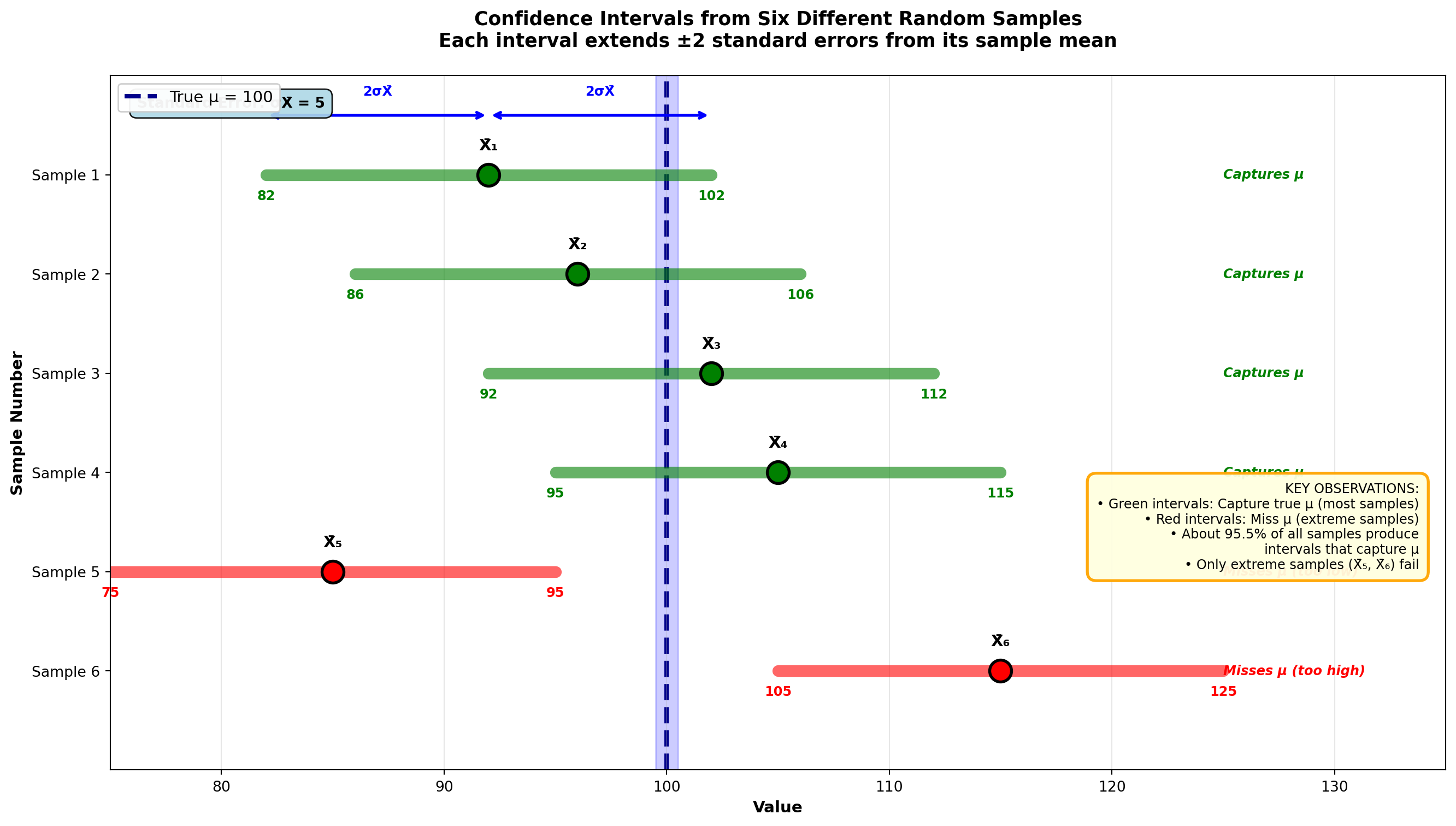
8.3.4 Determining the Z-Value for 95% Confidence
If we want to construct a more conventional 95% interval (rather than the 95.5% discussed above), how many standard errors should we move above and below the sample mean?
Because the standard normal (Z) table contains values only for the area that is above or below the mean, we must divide 95% by 2, producing 0.4750. Then we find the Z-value corresponding to an area of 0.4750, which is Z = 1.96.
Thus, to construct a 95% confidence interval, we simply specify an interval of 1.96 standard errors above and below the sample mean. This value of 95% is called the confidence coefficient.
Visual representation of 95% confidence interval:
Code
import matplotlib.pyplot as plt
import numpy as np
from scipy import stats

fig, ax = plt.subplots(figsize=(14, 7))

# Generate standard normal distribution
x = np.linspace(-4, 4, 1000)
y = stats.norm.pdf(x, 0, 1)

# Plot the distribution
ax.plot(x, y, 'b-', linewidth=3, label='Standard Normal Distribution')
ax.fill_between(x, y, alpha=0.2, color='blue')

# Shade the middle 95% (between -1.96 and +1.96)
x_middle = x[(x >= -1.96) & (x <= 1.96)]
y_middle = stats.norm.pdf(x_middle, 0, 1)
ax.fill_between(x_middle, y_middle, alpha=0.4, color='green',
                label='95% Confidence Region\n(Area = 0.95)')

# Shade the tails (rejection regions)
x_left = x[x < -1.96]
y_left = stats.norm.pdf(x_left, 0, 1)
ax.fill_between(x_left, y_left, alpha=0.4, color='red',
                label='Lower Tail (α/2 = 0.025)')

x_right = x[x > 1.96]
y_right = stats.norm.pdf(x_right, 0, 1)
ax.fill_between(x_right, y_right, alpha=0.4, color='red',
                label='Upper Tail (α/2 = 0.025)')

# Draw vertical lines at critical values
ax.axvline(-1.96, color='red', linestyle='--', linewidth=3, alpha=0.8)
ax.axvline(1.96, color='red', linestyle='--', linewidth=3, alpha=0.8)
ax.axvline(0, color='darkblue', linestyle='-', linewidth=2, alpha=0.6)

# Add labels for critical values
ax.text(-1.96, -0.02, 'Z = -1.96\n(LCL)', ha='center', fontsize=11,
        fontweight='bold', color='red',
        bbox=dict(boxstyle='round,pad=0.4', facecolor='lightcoral', alpha=0.9))
ax.text(1.96, -0.02, 'Z = +1.96\n(UCL)', ha='center', fontsize=11,
        fontweight='bold', color='red',
        bbox=dict(boxstyle='round,pad=0.4', facecolor='lightcoral', alpha=0.9))
ax.text(0, -0.02, 'Z = 0\n(μ)', ha='center', fontsize=11,
        fontweight='bold', color='darkblue',
        bbox=dict(boxstyle='round,pad=0.4', facecolor='lightblue', alpha=0.9))

# Add area labels
ax.text(0, 0.25, '0.4750', ha='center', fontsize=12, fontweight='bold',
        color='darkgreen',
        bbox=dict(boxstyle='round,pad=0.4', facecolor='lightgreen', alpha=0.8))
ax.text(-0.95, 0.25, '0.4750', ha='center', fontsize=12, fontweight='bold',
        color='darkgreen',
        bbox=dict(boxstyle='round,pad=0.4', facecolor='lightgreen', alpha=0.8))

ax.text(-2.8, 0.02, '0.025', ha='center', fontsize=10, fontweight='bold',
        color='darkred',
        bbox=dict(boxstyle='round,pad=0.3', facecolor='mistyrose', alpha=0.9))
ax.text(2.8, 0.02, '0.025', ha='center', fontsize=10, fontweight='bold',
        color='darkred',
        bbox=dict(boxstyle='round,pad=0.3', facecolor='mistyrose', alpha=0.9))

# Add arrows showing the middle area
ax.annotate('', xy=(-1.96, 0.15), xytext=(0, 0.15),
           arrowprops=dict(arrowstyle='<->', lw=3, color='darkgreen'))
ax.annotate('', xy=(1.96, 0.15), xytext=(0, 0.15),
           arrowprops=dict(arrowstyle='<->', lw=3, color='darkgreen'))

# Formatting
ax.set_title('95% Confidence Interval: Finding the Z-Value\n' +
             'Area = 0.95 split into two halves of 0.4750 each',
             fontsize=13, fontweight='bold', pad=15)
ax.set_xlabel('Z-value (Standard Deviations from Mean)', fontsize=11, fontweight='bold')
ax.set_ylabel('Probability Density', fontsize=11, fontweight='bold')
ax.set_xlim(-4, 4)
ax.set_ylim(-0.05, 0.45)
ax.grid(True, alpha=0.3, axis='x')
ax.legend(loc='upper left', fontsize=10, framealpha=0.95)

# Add explanation box
explanation = (
    "HOW TO FIND Z = 1.96:\n"
    "1. Confidence level = 95% = 0.95\n"
    "2. Divide by 2: 0.95 / 2 = 0.4750\n"
    "3. Look up 0.4750 in Z-table\n"
    "4. Result: Z = 1.96\n\n"
    "INTERPRETATION:\n"
    "• 95% of sample means fall within\n"
    "  ±1.96 standard errors of μ\n"
    "• Therefore, μ falls within ±1.96σX̄\n"
    "  of the sample mean for 95% of samples"
)
ax.text(0.98, 0.97, explanation, transform=ax.transAxes,
        fontsize=9, verticalalignment='top', horizontalalignment='right',
        bbox=dict(boxstyle='round,pad=0.7', facecolor='lightyellow',
                  edgecolor='orange', linewidth=2, alpha=0.95))

# Add total area label
ax.text(0, 0.38, 'Total Area = 0.95 (95% Confidence)',
        ha='center', fontsize=12, fontweight='bold', color='darkgreen',
        bbox=dict(boxstyle='round,pad=0.5', facecolor='lightgreen',
                  edgecolor='darkgreen', linewidth=2, alpha=0.9))

plt.tight_layout()
plt.show()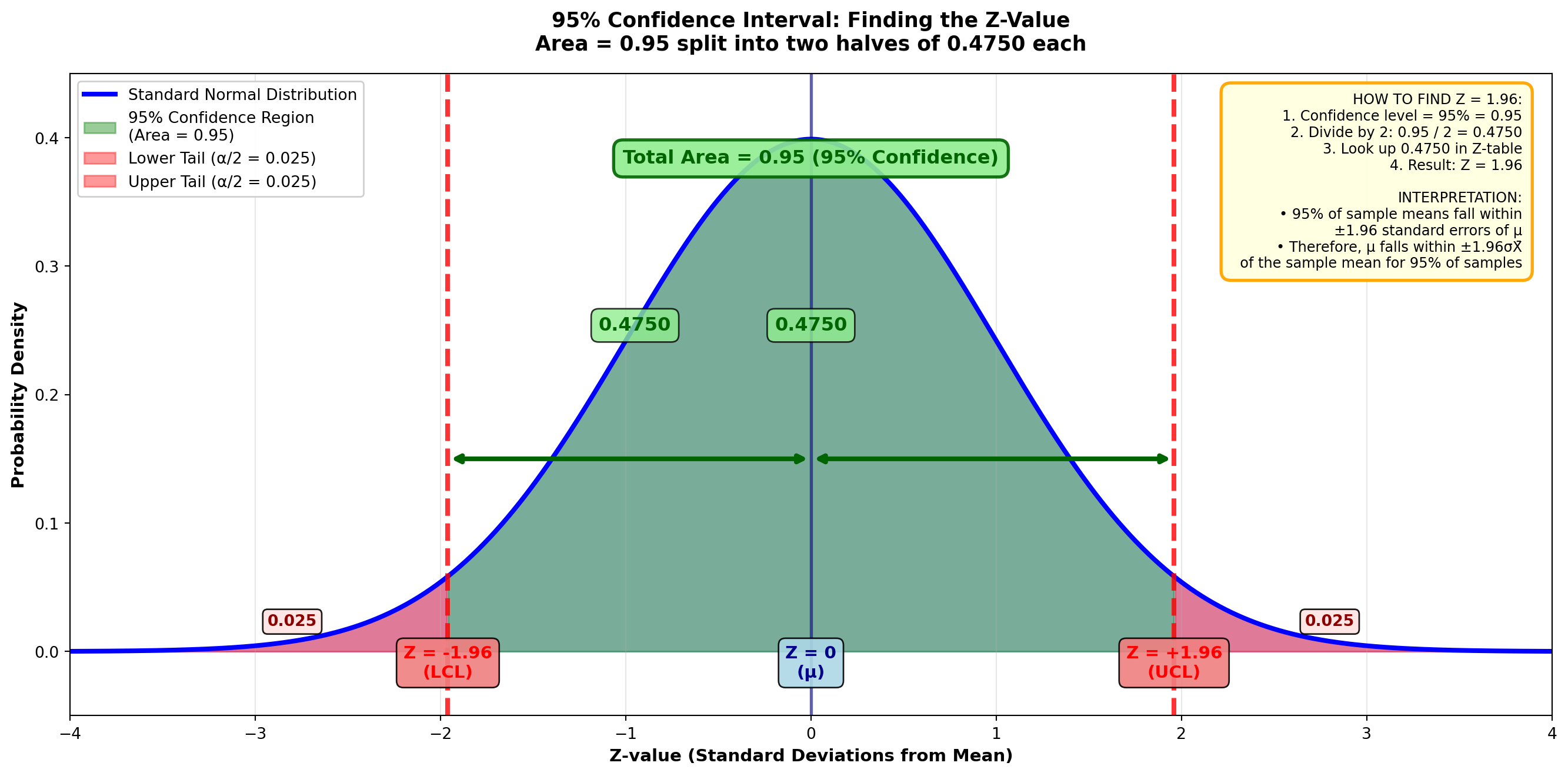
ImportantDefinition: Confidence Coefficient
The confidence coefficient is the level of confidence we have that the interval contains the unknown value of the parameter.
8.3.5 Common Confidence Levels and Their Z-Values
| Confidence Level | α | α/2 | Area from 0 to Z | Z-value |
|---|---|---|---|---|
| 90% | 0.10 | 0.05 | 0.4500 | 1.645 |
| 95% | 0.05 | 0.025 | 0.4750 | 1.96 |
| 99% | 0.01 | 0.005 | 0.4950 | 2.58 |
8.4 7.3 Confidence Intervals for the Population Mean: Large Samples
One of the most common uses of confidence intervals is to estimate the population mean. Examples include:
- A manufacturer estimating the average monthly output of a plant
- A marketing representative interested in the average weekly sales reduction
- A CFO of a Fortune 500 firm estimating average quarterly returns on corporate operations
The number of circumstances commonly encountered in the business world that require an estimate of the population mean is almost unlimited.
8.4.1 The General Formula (σ Known)
Recall that the interval is formed using the sample mean as a point estimate, to which we add and subtract a certain value to obtain the upper and lower limits of the confidence interval, respectively. Therefore, the interval is:
\text{C.I. for } \mu = \bar{X} \pm Z\sigma_{\bar{X}} \tag{8.1}
where \sigma_{\bar{X}} = \frac{\sigma}{\sqrt{n}} is the standard error of the mean.
How much should be added and subtracted depends in part on the desired confidence level, stipulated by the value of Z in the formula. A 95% confidence level requires a Z-value of 1.96 (since 0.95/2 = 0.4750, and the area of 0.4750 corresponds to Z = 1.96).
8.4.2 Example 7.2: Real Estate Development Income Study
A real estate developer is trying to build a large shopping center. He wants to estimate the average income per family in the area as an indicator of expected sales. A sample of n = 100 families yields a mean of \bar{X} = \$35,500. Assume the population standard deviation is \sigma = \$7,200.
Solution:
Given that \sigma_{\bar{X}} = \frac{\sigma}{\sqrt{n}} = \frac{7,200}{\sqrt{100}} = \$720, we estimate a 95% interval as:
\begin{aligned} \text{C.I. for } \mu &= 35,500 \pm (1.96)\frac{7,200}{\sqrt{100}} \\ &= 35,500 \pm 1,411.20 \\ &= \$34,088.80 \leq \mu \leq \$36,911.20 \end{aligned}
Interpretation:
The developer can be 95% confident that the true unknown population mean income is between \$34,088.80 and \$36,911.20. While the actual value for the population mean remains unknown, the developer has 95% confidence that it lies between these two values.
TipBusiness Application
This interval provides the developer with critical information for investment decisions. If the shopping center’s business plan requires average family incomes of at least \$33,000, the developer can proceed with confidence. However, if financing requires demonstrated incomes above \$37,000, the current data suggest the market may not support the development.
8.5 7.4 Interpreting Confidence Intervals
There are two valid interpretations of a confidence interval. Understanding both deepens comprehension of what confidence intervals actually tell us.
8.5.1 Interpretation 1: The Confidence Statement (Most Common)
The first, and most common interpretation, states that the developer has “95% confidence that the true unknown population mean is between \$34,088.80 and \$36,911.20.”
Although the actual value for the population mean remains unknown, the developer has 95% confidence that it lies between these two values. This is the practical interpretation used in business decision-making.
8.5.2 Interpretation 2: The Long-Run Frequency Interpretation
The second interpretation recognizes that many different confidence intervals could be developed. Another sample would probably produce a different sample mean due to sampling error. With a different \bar{X}, the interval would have different upper and lower limits.
Therefore, the second interpretation states: If we constructed all possible confidence intervals (one from each possible sample), 95% of them would contain the unknown population mean.
8.5.3 Example 7.3: Comparing Two Confidence Intervals
If a second sample yields a mean of \$35,600 instead of \$35,500, the interval becomes:
\begin{aligned} \text{C.I. for } \mu &= \$35,600 \pm (1.96)\frac{\$7,200}{\sqrt{100}} \\ &= \$34,188.80 \leq \mu \leq \$37,011.20 \end{aligned}
The developer can be 95% sure that the population mean is between \$34,188.80 and \$37,011.20. If all possible intervals were constructed based on all the different possible sample means, 95% of them would contain the unknown population mean.
8.5.4 The Alpha Value: Probability of Error
This, of course, means that 5% of all intervals would be wrong — they would not contain the population mean. This 5%, found as (1 - confidence coefficient), is called the alpha value (α) and represents the probability of error.
WarningDefinition: Alpha Value (α)
The alpha value is the probability of error, or the probability that any given interval does not contain the unknown population mean.
\alpha = 1 - \text{Confidence Coefficient}
For a 95% confidence interval: \alpha = 1 - 0.95 = 0.05
Visual representation:
If we construct 100 different 95% confidence intervals:
- Approximately 95 will contain μ ✓
- Approximately 5 will NOT contain μ ✗

This is what "95% confidence" means!
8.6 7.5 Confidence Intervals When σ is Unknown
8.6.1 The Practical Reality
Formula Equation 8.1 requires the unlikely assumption that the population standard deviation \sigma is known. In the likely event that \sigma is unknown, the sample standard deviation must be substituted:
\text{C.I. for } \mu = \bar{X} \pm Zs_{\bar{X}} \tag{8.2}
where s_{\bar{X}} = \frac{s}{\sqrt{n}} is the estimated standard error of the mean.
8.6.2 Example 7.4: CPA Tax Returns Study
Gerry Gerber, CPA, has just filed the tax returns for his clients. He wants to estimate the average amount owed to the Internal Revenue Service (IRS). Of the 50 clients he selected in his sample, the average amount owed was \bar{X} = \$652.68.
Since the standard deviation of all his clients (\sigma) is unknown, Gerber must estimate \sigma with the sample standard deviation of s = \$217.43.
Solution (99% confidence level):
If a 99% confidence level is desired, the appropriate Z-value is 2.58 (since 0.99/2 = 0.4950, and from the Z-table, an area of 0.4950 reveals Z = 2.58).
Using formula Equation 8.2:
\begin{aligned} \text{C.I. for } \mu &= \bar{X} \pm Zs_{\bar{X}} \\ &= \$652.68 \pm 2.58\frac{\$217.43}{\sqrt{50}} \\ &= \$652.68 \pm 79.33 \\ &= \$573.35 \leq \mu \leq \$732.01 \end{aligned}
Interpretation:
Mr. Gerber can be 99% confident that the average amount owed by all his clients to the IRS is between \$573.35 and \$732.01.
8.6.3 Trading Confidence for Precision
What would happen to this interval if Mr. Gerber were willing to accept a 95% confidence level? With a Z-value of 1.96, the interval would be:
\begin{aligned} \text{C.I. for } \mu &= \$652.68 \pm 1.96\frac{\$217.43}{\sqrt{50}} \\ &= \$652.68 \pm 60.27 \\ &= \$592.41 \leq \mu \leq \$712.95 \end{aligned}
The results are both good and bad:
NoteGood News: More Precision
The 95% interval is narrower and offers greater precision. A wide interval is not especially useful. It would reveal very little if your professor told you the mean on the next exam would be between 0 and 100%. The narrower the interval, the more meaningful it is.
WarningBad News: Less Confidence
Mr. Gerber is now only 95% sure that the interval actually contains \mu. Although the interval is more precise (narrower), the probability that it contains \mu has been reduced from 99% to 95%. Mr. Gerber had to give up some confidence to gain more precision.
8.6.4 Comparison Table: 99% vs 95% Confidence
| Confidence Level | Z-value | Margin of Error | Interval Width | LCL | UCL |
|---|---|---|---|---|---|
| 99% | 2.58 | $79.33 | $158.66 | $573.35 | $732.01 |
| 95% | 1.96 | $60.27 | $120.54 | $592.41 | $712.95 |
Key insight: There is always a trade-off between confidence and precision. Higher confidence requires a wider interval; narrower intervals come at the cost of lower confidence.
END OF STAGE 1
This completes sections 7.1-7.5 covering: - Introduction to interval estimation - Foundation and logic of confidence intervals - Large sample confidence intervals for means - Interpretation of confidence intervals - Handling unknown population standard deviation
Next stage will cover: Small samples and the t-distribution (7.6), and confidence intervals for proportions (7.7). ## 7.6 Confidence Intervals for Small Samples: The t-Distribution {#sec-ci-small-samples}
8.6.5 When Large Samples Aren’t Possible
In all the previous examples, the sample size was large (n \geq 30). However, it’s not always possible to obtain at least 30 observations:
- An insurance company testing the impact resistance of luxury cars may find it prohibitively expensive to deliberately destroy 30 vehicles
- A medical researcher testing a new medicine may not find 30 people willing to act as guinea pigs
- Time constraints may limit data collection
- Population sizes may be inherently small
In many cases, a large sample is simply not feasible.
8.6.6 When to Use the t-Distribution
When a small sample must be taken, the normal distribution may not apply. The Central Limit Theorem ensures normality in the sampling process only if the sample is large. When using a small sample, an alternative distribution may be necessary: the t-distribution (or Student’s t-distribution).
ImportantThree Conditions for Using the t-Distribution
The t-distribution is used when all three conditions are met:
- The sample is small (n < 30)
- \sigma is unknown (must use s)
- The population is normal or nearly normal
Important notes: - If \sigma is known, use the Z-distribution even if the sample is small - If a normal population cannot be assumed, increase the sample size to use the Z-distribution - If neither option is possible, rely on non-parametric tests
8.6.7 Historical Background: William S. Gosset and “Student”
The Student’s t-distribution was developed in 1908 by William S. Gosset (1876-1937), who worked as a master brewer for Guinness Breweries in Dublin, Ireland. Guinness did not allow its employees to publish their research, so Gosset (who liked to “play with numbers to relax”) first reported his t-distribution under the pseudonym “Student” to protect his employment.
This is why we call it “Student’s t-distribution” today—a tribute to Gosset’s clever workaround and his fundamental contribution to statistics.
8.6.8 Properties of the t-Distribution
Similarities to the normal (Z) distribution: - Mean of zero - Symmetric about the mean - Ranges from -\infty to +\infty
Key difference: While the Z-distribution has a variance of \sigma^2 = 1, the variance of the t-distribution is greater than 1. Therefore, it is flatter and more spread out than the Z-distribution.
The variance for the t-distribution is:
\sigma^2 = \frac{n-1}{n-3} \tag{8.3}
where n-1 represents the degrees of freedom (d.f.).
8.6.9 Understanding Degrees of Freedom
NoteDefinition: Degrees of Freedom
Degrees of freedom (d.f.) is defined as the number of observations that can be chosen freely. It equals the number of observations minus the number of restrictions imposed on those observations, where a restriction is some value that those observations must possess.
Example: Suppose you have n = 4 observations that must produce a mean of 10. The mean of 10 serves as a restriction, and there are n - 1 = 3 degrees of freedom.
You can choose three observations freely; for example, you can choose 8, 9, and 11. After these three values are selected, there is no freedom to choose the last observation. The fourth value must be 12 if you want to have an average of 10.
\frac{8 + 9 + 11 + 12}{4} = \frac{40}{4} = 10 \checkmark
8.6.10 The Family of t-Distributions
The t-distribution is actually a family of distributions, each with its own variance. The variance depends on the degrees of freedom.
Code
import matplotlib.pyplot as plt
import numpy as np
from scipy import stats

fig, ax = plt.subplots(figsize=(12, 7))

# Generate x values
x = np.linspace(-4, 4, 1000)

# Standard Normal (Z) distribution
z_dist = stats.norm(0, 1)
y_z = z_dist.pdf(x)

# t-distributions with different degrees of freedom
df_values = [5, 10, 30]
colors = ['red', 'orange', 'green']
labels = ['t (d.f. = 5)', 't (d.f. = 10)', 't (d.f. = 30)']

# Plot t-distributions
for df, color, label in zip(df_values, colors, labels):
    t_dist = stats.t(df)
    y_t = t_dist.pdf(x)
    ax.plot(x, y_t, color=color, linewidth=2.5, label=label, alpha=0.8)
    ax.fill_between(x, y_t, alpha=0.15, color=color)

# Plot standard normal last (on top)
ax.plot(x, y_z, 'b-', linewidth=3, label='Standard Normal (Z)', zorder=10)
ax.fill_between(x, y_z, alpha=0.2, color='blue', zorder=5)

# Add annotations showing the differences
ax.annotate('Heavier tails\n(more spread)',
           xy=(-2.5, 0.05), xytext=(-3.5, 0.15),
           arrowprops=dict(arrowstyle='->', lw=2, color='red'),
           fontsize=10, fontweight='bold',
           bbox=dict(boxstyle='round,pad=0.5', facecolor='lightcoral', alpha=0.8))

ax.annotate('Approaching\nnormal as d.f.\nincreases',
           xy=(0, 0.35), xytext=(1.5, 0.35),
           arrowprops=dict(arrowstyle='->', lw=2, color='green'),
           fontsize=10, fontweight='bold',
           bbox=dict(boxstyle='round,pad=0.5', facecolor='lightgreen', alpha=0.8))

# Mark the peak difference
ax.plot([0, 0], [0, 0.4], 'k--', linewidth=1, alpha=0.5)
ax.text(0.1, 0.42, 'All centered\nat μ = 0', fontsize=9, fontweight='bold')

# Formatting
ax.set_title('t-Distribution Family: Effect of Degrees of Freedom\nAs d.f. → ∞, t-distribution → Normal distribution',
            fontsize=13, fontweight='bold')
ax.set_xlabel('Value', fontsize=11, fontweight='bold')
ax.set_ylabel('Probability Density', fontsize=11, fontweight='bold')
ax.legend(loc='upper right', fontsize=10, framealpha=0.9)
ax.grid(True, alpha=0.3)
ax.set_xlim(-4, 4)
ax.set_ylim(0, 0.45)

# Add comparison table as text
table_text = (
    "Key Characteristics:\n"
    "• Lower d.f. = Flatter, heavier tails\n"
    "• Higher d.f. = Closer to normal\n"
    "• d.f. ≥ 30 ≈ Normal (use Z)\n"
    "• All symmetric around μ = 0"
)
ax.text(0.02, 0.97, table_text, transform=ax.transAxes,
       fontsize=9, verticalalignment='top',
       bbox=dict(boxstyle='round,pad=0.5', facecolor='lightyellow', alpha=0.9))

plt.tight_layout()
plt.show()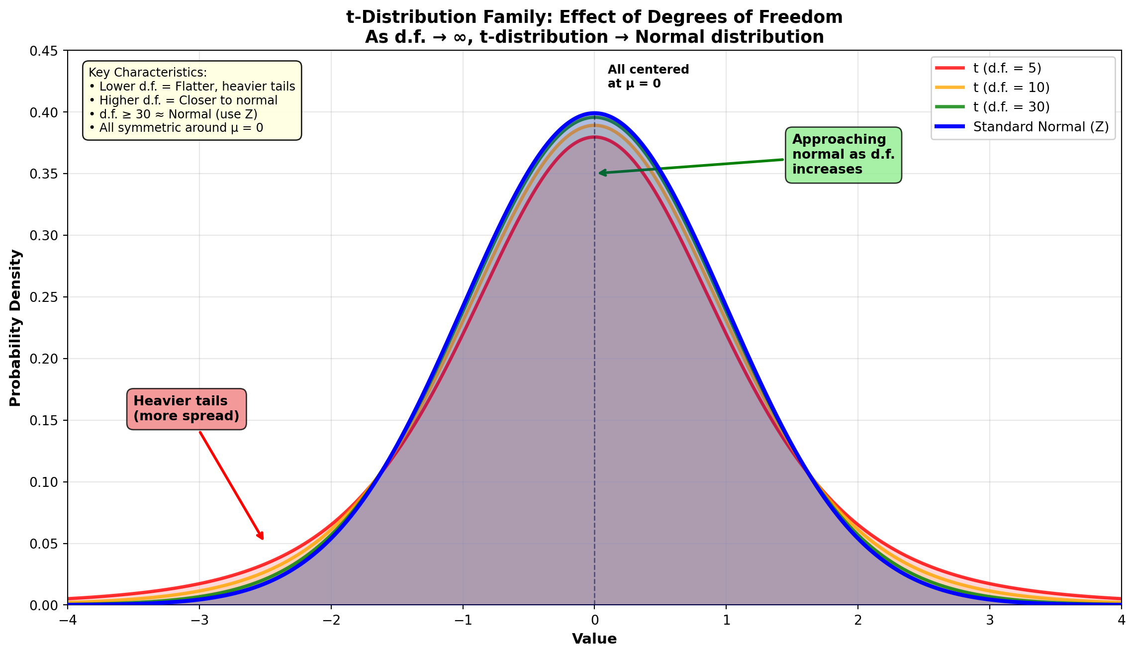
Important observation: As shown in the figure above, as n increases, the t-distribution approaches the normal (Z) distribution. This is why we can use the Z-distribution when n \geq 30.
8.6.11 Computing the t-Statistic
The t-statistic is calculated much like the Z-statistic:
t = \frac{\bar{X} - \mu}{s_{\bar{X}}} \tag{8.4}
where s_{\bar{X}} = \frac{s}{\sqrt{n}} is the estimated standard error.
Rewriting algebraically to express it as a confidence interval for estimating \mu:
\text{C.I. for } \mu = \bar{X} \pm (t)(s_{\bar{X}}) = \bar{X} \pm t\frac{s}{\sqrt{n}} \tag{8.5}
8.6.12 Using the t-Table
The appropriate value of t can be found from the t-table (Appendix F). To illustrate, assume you want a 95% confidence interval and have a sample of 20 observations.
Steps: 1. Calculate degrees of freedom: d.f. = n - 1 = 20 - 1 = 19 2. Go down the first column under “d.f.” to 19 3. Move across that row to the column headed by a confidence level of 0.95 for two-tailed tests 4. The resulting entry of 2.093 is the appropriate t-value
Note: Ignore the two rows referring to one-tailed tests; these will be covered in Chapter 8 on hypothesis testing.
8.6.13 Example 7.5: Construction Company Legal Case
Consider this problem taken from The Wall Street Journal. A construction company was accused of inflating vouchers it recorded for construction contracts with the federal government. The contract stipulated that a certain type of work should average \$1,150.
Due to time constraints, managers from only 12 government agencies were called to testify in court regarding the company’s vouchers. If the testimony revealed a mean of \bar{X} = \$1,275 and a standard deviation of s = \$235, would a 95% confidence interval support the company’s legal case? Assume the voucher amounts are normally distributed.
Solution:
A 95% confidence level with d.f. = 12 - 1 = 11 yields from the t-table a value of t = 2.201. Therefore:
\begin{aligned} \text{C.I. for } \mu &= \bar{X} \pm t\frac{s}{\sqrt{n}} \\ &= 1,275 \pm (2.201)\frac{235}{\sqrt{12}} \\ &= 1,275 \pm 149.31 \\ &= \$1,125.69 \leq \mu \leq \$1,424.31 \end{aligned}
Interpretation:
The court can be 95% confident that the average of all vouchers is between \$1,125 and \$1,424. This interval contains the agreed-upon \$1,150, strengthening the company’s defense. The data do not provide evidence of systematic overcharging.
TipLegal and Business Implications
This case illustrates how confidence intervals can be used in legal proceedings. Because the contractual amount (\$1,150) falls within the 95% confidence interval, the company has statistical evidence that their average billing is consistent with the contract terms. The variation observed could be explained by normal sampling variation rather than fraudulent inflation.
8.6.14 Comparing t-Values to Z-Values
It’s worth noting that the t-value for a 95% interval is 2.201 (given d.f. = 11), while a 95% interval from a large sample uses a Z-value of 1.96. The interval based on a t-value is therefore wider.
This additional width is necessary because we lose some precision when \sigma is unknown and must be estimated with s.
| Distribution | Value | Interval Width | Reason |
|---|---|---|---|
| Z (large n, σ known) | 1.96 | Narrower | Maximum information |
| t (small n, σ unknown) | 2.201 | Wider | Accounts for additional uncertainty |
8.6.15 Example 7.6: United Auto Workers Production Standards
The labor contract between United Auto Workers (UAW) and Ford Motor Company (FMC) required that average production for a production section be maintained at 112 units per month, per employee. Disagreements arose between UAW and FMC regarding whether this standard was being maintained.
The labor contract specified that if average production levels fell below the stipulated amount of \mu = 112, FMC would be allowed to take “corrective actions.” Due to the cost involved, only 20 workers were evaluated, resulting in a mean of 102 units. Assume a standard deviation of 8.5 units was found and that production levels are normally distributed.
Would a 90% confidence interval tend to suggest a violation of the labor contract, thus allowing corrective action?
Solution:
With a 90% confidence level and n - 1 = 19 degrees of freedom, the t-table gives a t-value of 1.729.
\begin{aligned} \text{C.I. for } \mu &= \bar{X} \pm t\frac{s}{\sqrt{n}} \\ &= 102 \pm (1.729)\frac{8.5}{\sqrt{20}} \\ &= 102 \pm 3.29 \\ &= 98.71 \leq \mu \leq 105.29 \end{aligned}
Interpretation:
The production level average of 112 units, specified in the labor contract, is not within the confidence interval. There is a 90% confidence level that the contract is being violated. FMC is within its rights to pursue a remedy for delayed productivity.
WarningManagement Decision Point
This example shows how confidence intervals inform labor relations decisions. The statistical evidence (with 90% confidence) suggests production has fallen below contractual levels, providing objective grounds for management intervention. However, management must also consider:
- Whether 90% confidence is sufficient for such consequential decisions
- Root causes of the productivity decline
- Potential impacts of corrective actions on labor relations
8.6.16 Decision Tree: Choosing Between Z and t
Deciding whether to use a t-statistic or Z-statistic is crucial. The following decision tree helps in selecting the appropriate statistic:
graph TD
    A[Start: Estimate μ] --> B{Is n ≥ 30?}
    B -->|Yes| C{Is σ known?}
    B -->|No| D{Is population normal?}

    C -->|Yes| E[Use Z with σ]
    C -->|No| F[Use Z with s]

    D -->|Yes| G{Is σ known?}
    D -->|No| H[Cannot use CI<br/>Consider:<br/>- Increase n<br/>- Use nonparametric]

    G -->|Yes| I[Use Z with σ]
    G -->|No| J[Use t with s]

    style E fill:#90EE90
    style F fill:#90EE90
    style I fill:#90EE90
    style J fill:#FFD700
    style H fill:#FFB6C6
ImportantQuick Reference: When to Use t vs. Z
Use the t-distribution when ALL THREE conditions are met: 1. Population is normal ✓ 2. Small sample (n < 30) ✓ 3. \sigma is unknown ✓
Otherwise, use the Z-distribution or alternative methods.
8.6.17 Section Exercises
Exercise 7.1: The Lucky Lady, a popular student hangout, sells 16-ounce glasses of beer. Ten students purchase a total of 22 glasses, and using their own measuring cup, estimate the contents on average. The sample mean is 15.2 ounces, with s = 0.86. With a 95% confidence level, do the students believe their money is well spent? Interpret the interval.
Exercise 7.2: Dell Publishing samples 23 packages to estimate average postal cost. The sample mean is \bar{X} = \$23.56, with s = \$4.65.
- The senior editor at Dell hopes to keep average cost below \$23.00. Calculate and interpret the 99% confidence interval. Will the editor be satisfied?
- Compare the results of part (a) with the 99% confidence interval if s = \$2.05. Explain why there is a difference.
- Keeping s = \$4.65, compare the results of part (a) with the 95% interval. Explain the difference.
Exercise 7.3: Bonuses for 10 new players in the National Football League are used to estimate the average bonus for all new players. The sample mean is \$65,890 with s = \$12,300. What is your estimate with a 90% interval for the population mean?
8.7 7.7 Confidence Intervals for Population Proportions
8.7.1 Binary Outcomes in Business Decisions
Decisions frequently depend on parameters that are binary—parameters with only two possible categories into which responses can be classified. In this event, the parameter of interest is the population proportion.
Common business applications:
- What proportion of customers pay by credit vs. cash?
- What percentage of products are defective vs. non-defective?
- What proportion of employees quit after one year vs. stay?
- What percentage of voters support vs. oppose a policy?
In each of these cases, there are only two possible outcomes. Therefore, the concern focuses on the proportion of responses that fall within one of these two outcomes.
8.7.2 The Standard Error for Proportions
In Chapter 6, we found that if n\pi and n(1-\pi) are both greater than 5, the distribution of sample proportions will be normal, and the sampling distribution of the sample proportion will have:
- A mean equal to the population proportion \pi
- A standard error of:
\sigma_p = \sqrt{\frac{\pi(1-\pi)}{n}} \tag{8.6}
However, this formula contains \pi, the parameter we’re trying to estimate! Therefore, the sample proportion p is used as an estimator of \pi.
The formula can be restated as:
s_p = \sqrt{\frac{p(1-p)}{n}} \tag{8.7}
8.7.3 The Confidence Interval Formula for Proportions
The confidence interval is then:
\text{C.I. for } \pi = p \pm Zs_p \tag{8.8}
where p = \frac{X}{n} is the sample proportion, X is the number of “successes” in the sample, and n is the sample size.
8.7.4 Example 7.7: Television Station Market Research
The manager of a television station must determine what percentage of households in the city have more than one television. A random sample of 500 households reveals that 275 have two or more televisions.
What is the 90% confidence interval for estimating the proportion of all households that have two or more televisions?
Solution:
Given these data, p = \frac{275}{500} = 0.55, and:
s_p = \sqrt{\frac{(0.55)(0.45)}{500}} = \sqrt{\frac{0.2475}{500}} = 0.022
The Z-table gives a value of Z = 1.65 for a 90% confidence interval (0.90/2 = 0.45 area).
\begin{aligned} \text{C.I. for } \pi &= 0.55 \pm (1.65)(0.022) \\ &= 0.55 \pm 0.036 \\ &= 0.514 \leq \pi \leq 0.586 \end{aligned}
Interpretation:
The manager can be 90% confident that between 51.4% and 58.6% of households in the city have more than one television.
TipBusiness Application: Advertising Strategy
This information is valuable for the station’s advertising sales team. They can confidently tell potential advertisers that roughly 51-59% of households have multiple TVs, suggesting:
- Potential for simultaneous viewing by different family members
- Opportunity for targeted programming on multiple channels
- Market segmentation strategies based on multi-TV ownership
8.7.5 Example 7.8: Executive Search Firms and Outside CEOs
Executive search firms (“headhunters”) specialize in helping companies locate and secure top management talent. Business Week recently reported that “one in four CEOs is an outsider—an executive with less than 5 years at the company they manage.”
If in a sample of 350 companies in the United States, 77 have outside CEOs, would a 99% confidence interval support this claim?
Solution:
\begin{aligned} p &= \frac{77}{350} = 0.22 \\ s_p &= \sqrt{\frac{(0.22)(0.78)}{350}} = 0.022 \end{aligned}
For a 99% confidence interval, Z = 2.58:
\begin{aligned} \text{C.I. for } \pi &= p \pm Zs_p \\ &= 0.22 \pm (2.58)(0.022) \\ &= 0.22 \pm 0.057 \\ &= 0.163 \leq \pi \leq 0.277 \end{aligned}
Interpretation:
We are confident at the 99% level that between 16.3% and 27.7% of U.S. companies have outside CEOs. The claim is supported by these findings, since 25% (one in four) is contained within the interval.
NoteVerification of Claims
This example illustrates how confidence intervals can verify or refute published claims. The Business Week assertion of “one in four” (25%) falls comfortably within our 99% confidence interval, providing statistical support for their reporting.
8.7.6 Example 7.9: National Travel Association Tourism Study
The National Travel Association sampled people taking vacations in Ireland to estimate the frequency with which North Americans visit the Emerald Isle.
Part (a): What is the 96% confidence interval for the proportion of tourists who are North Americans, if 1,098 of the 3,769 surveyed carried U.S. passports?
Solution:
\begin{aligned} p &= \frac{1,098}{3,769} = 0.2913 \\ s_p &= \sqrt{\frac{(0.2913)(0.7087)}{3,769}} = 0.0074 \end{aligned}
For 96% confidence, we need the Z-value where the area from 0 to Z is 0.48. From the Z-table: Z = 2.05.
\begin{aligned} \text{C.I. for } \pi &= 0.2913 \pm (2.05)(0.0074) \\ &= 0.2913 \pm 0.0152 \\ &= 0.2761 \leq \pi \leq 0.3065 \end{aligned}
Interpretation: With 96% confidence, between 27.61% and 30.65% of all tourists to Ireland are North Americans.
Part (b): Of the 1,098 North American tourists, 684 had booked their trip through a travel agent. Calculate and interpret the 95% interval for the proportion of all North Americans who use professional travel agency services in Ireland.
Solution:
\begin{aligned} p &= \frac{684}{1,098} = 0.6230 \\ s_p &= \sqrt{\frac{(0.6230)(0.3770)}{1,098}} = 0.0146 \end{aligned}
For 95% confidence, Z = 1.96:
\begin{aligned} \text{C.I. for } \pi &= 0.6230 \pm (1.96)(0.0146) \\ &= 0.6230 \pm 0.0286 \\ &= 0.5944 \leq \pi \leq 0.6516 \end{aligned}
Interpretation: With 95% confidence, between 59.44% and 65.16% of North American tourists to Ireland use travel agents.
TipIndustry Insights
These findings are valuable for:
Travel agencies: Strong evidence (roughly 60-65%) that their services remain important for international travel, despite online booking options
Irish tourism board: Understanding that approximately 28-31% of tourists are North American helps in targeted marketing campaigns
Airlines: Route planning and capacity decisions can be informed by these proportions
8.7.7 Summary: Proportions vs. Means
| Aspect | Population Mean (μ) | Population Proportion (π) |
|---|---|---|
| Parameter | \mu | \pi |
| Point Estimate | \bar{X} | p = X/n |
| Standard Error (pop.) | \sigma_{\bar{X}} = \frac{\sigma}{\sqrt{n}} | \sigma_p = \sqrt{\frac{\pi(1-\pi)}{n}} |
| Standard Error (sample) | s_{\bar{X}} = \frac{s}{\sqrt{n}} | s_p = \sqrt{\frac{p(1-p)}{n}} |
| Interval (large n) | \bar{X} \pm Zs_{\bar{X}} | p \pm Zs_p |
| Interval (small n) | \bar{X} \pm ts_{\bar{X}} | Not used (need n\pi > 5) |
8.7.8 Section Exercises
Exercise 7.4: What is s_p and what does it measure?
Exercise 7.5: CNN reported that 68% of all high school students have computers in their homes. If a sample of 1,020 students reveals that 673 have home computers, does a 99% interval support CNN?
Exercise 7.6: In response to the new cigarette smoking craze sweeping the nation, the National Heart Institute surveyed women to estimate the proportion who smoke cigarettes occasionally. Of the 750 women who responded, 287 said they did. Based on these data, what is your 90% estimate for the proportion of all women who participate in this habit?
END OF STAGE 2
This completes sections 7.6-7.7 covering: - Small sample confidence intervals using the t-distribution - Degrees of freedom concept - Decision tree for choosing t vs. Z - Confidence intervals for population proportions - Multiple business examples (construction, labor contracts, CEOs, tourism)
Next stage will cover: Controlling interval width (7.8), sample size determination (7.9), and properties of estimators (7.10). ## 7.8 Controlling the Width of an Interval {#sec-ci-width-control}
As stated earlier, a narrower interval is preferable due to the additional precision it provides. There are two main methods to achieve a more precise interval:
- Reduce the confidence level
- Increase the sample size
8.7.9 Method 1: Reducing the Confidence Level
We’ve already seen, in Mr. Gerber’s attempt to estimate the average tax return of his clients, that an increase in precision can be obtained by accepting a lower confidence level.
Recall Example 7.4 (Gerber’s CPA Tax Returns):
- Sample: n = 50 clients
- Sample mean: \bar{X} = \$652.68
- Sample standard deviation: s = \$217.43
99% Confidence Interval:
\text{C.I.} = \$652.68 \pm 2.58\frac{\$217.43}{\sqrt{50}} = \$573.35 \text{ to } \$732.01
Interval width: \$732.01 - \$573.35 = \$158.66
95% Confidence Interval:
\text{C.I.} = \$652.68 \pm 1.96\frac{\$217.43}{\sqrt{50}} = \$592.41 \text{ to } \$712.95
Interval width: \$712.95 - \$592.41 = \$120.54
The 95% interval is narrower ($120.54 vs. $158.66), providing greater precision. This resulted from the fact that the 99% confidence interval required a Z-value of 2.58 instead of 1.96.
WarningThe Cost of Precision
However, there was a cost involved in achieving this greater precision: the confidence level dropped to 95%, producing a 5% probability of error instead of the 1% related to the 99% confidence interval.
The fundamental trade-off: - More precision (narrower interval) → Less confidence - More confidence (wider interval) → Less precision
Is there a way to reduce the interval without suffering a loss of confidence? Yes! By increasing the sample size.
8.7.10 Method 2: Increasing the Sample Size
By increasing the sample size, we can reduce the standard error \frac{\sigma}{\sqrt{n}} or \frac{s}{\sqrt{n}}. The standard error appears in the denominator with \sqrt{n}, so as n increases, the standard error decreases.
If Mr. Gerber’s sample size is increased to n = 80, the 99% interval presents a degree of precision similar to the narrower 95% interval, without any loss of confidence.
With n = 80, the 99% interval is:
\begin{aligned} \text{C.I. for } \mu &= \$652.68 \pm 2.58\frac{\$217.43}{\sqrt{80}} \\ &= \$652.68 \pm 62.71 \\ &= \$589.97 \leq \mu \leq \$715.39 \end{aligned}
Interval width: \$715.39 - \$589.97 = \$125.42
This is very close to the more precise 95% interval of \$592.41 to \$712.95 (width = $120.54), but maintains a 99% confidence level!
8.7.11 Comparison of Methods
| Method | n | Confidence | Z-value | Width | Interpretation |
|---|---|---|---|---|---|
| Original | 50 | 99% | 2.58 | $158.66 | Wide, high confidence |
| Reduce confidence | 50 | 95% | 1.96 | $120.54 | Narrow, lower confidence |
| Increase sample | 80 | 99% | 2.58 | $125.42 | Narrow, high confidence ✓ |
TipBest of Both Worlds
By increasing the sample size from 50 to 80, Mr. Gerber achieved: - Similar precision to the 95% interval - Maintained the higher 99% confidence level - No trade-off in confidence for precision
8.7.12 The Price of Larger Samples
Unfortunately, this advantage is not gained without a price. The larger sample size means more time and more money must be spent collecting and handling the data. Once again, a decision must be made—it becomes a managerial decision regarding which method to take.
Managerial considerations:
- Budget constraints: Is additional data collection affordable?
- Time pressures: Is there sufficient time to collect more data?
- Marginal value: Does the precision gain justify the additional cost?
- Decision criticality: How important is high confidence vs. precision for this specific decision?
8.7.13 Visual Representation of Interval Width Control
Code
import matplotlib.pyplot as plt
import numpy as np

fig, axes = plt.subplots(2, 1, figsize=(14, 10))

# Common parameters
sample_mean = 100
sigma = 15

# Panel 1: Effect of Confidence Level (n fixed at 50)
n_fixed = 50
se_fixed = sigma / np.sqrt(n_fixed)

confidence_levels = [90, 95, 99]
z_values = [1.645, 1.96, 2.58]
colors_conf = ['green', 'orange', 'red']

for i, (conf, z, color) in enumerate(zip(confidence_levels, z_values, colors_conf)):
    margin = z * se_fixed
    lcl = sample_mean - margin
    ucl = sample_mean + margin

    # Draw interval
    y_pos = 2 - i * 0.7
    axes[0].plot([lcl, ucl], [y_pos, y_pos], color=color, linewidth=8,
                solid_capstyle='round', label=f'{conf}% CI (Z={z})')

    # Draw center point
    axes[0].plot(sample_mean, y_pos, 'ko', markersize=10, zorder=5)

    # Add interval width annotation
    axes[0].text(sample_mean, y_pos + 0.15, f'Width = {2*margin:.2f}',
                ha='center', fontsize=9, fontweight='bold',
                bbox=dict(boxstyle='round,pad=0.3', facecolor=color, alpha=0.3))

# Formatting Panel 1
axes[0].axvline(sample_mean, color='blue', linestyle='--', linewidth=2, alpha=0.5,
               label='Sample Mean (X̄)')
axes[0].set_title('Effect of Confidence Level on Interval Width\n(n = 50 fixed, σ = 15)',
                 fontsize=13, fontweight='bold')
axes[0].set_xlabel('Value', fontsize=11, fontweight='bold')
axes[0].set_yticks([2, 1.3, 0.6])
axes[0].set_yticklabels(['90% CI\n(Narrowest)', '95% CI\n(Moderate)', '99% CI\n(Widest)'])
axes[0].legend(loc='upper left', fontsize=10)
axes[0].grid(True, alpha=0.3, axis='x')
axes[0].set_xlim(85, 115)
axes[0].set_ylim(-0.2, 2.5)

# Add key insight
axes[0].text(0.98, 0.95,
            'KEY INSIGHT:\nHigher confidence\n→ Wider interval\n→ Less precision',
            transform=axes[0].transAxes, fontsize=10, fontweight='bold',
            verticalalignment='top', horizontalalignment='right',
            bbox=dict(boxstyle='round,pad=0.5', facecolor='yellow', alpha=0.9))

# Panel 2: Effect of Sample Size (95% confidence fixed)
z_fixed = 1.96
sample_sizes = [25, 50, 100, 200]
colors_n = ['red', 'orange', 'yellow', 'green']

for i, (n, color) in enumerate(zip(sample_sizes, colors_n)):
    se = sigma / np.sqrt(n)
    margin = z_fixed * se
    lcl = sample_mean - margin
    ucl = sample_mean + margin

    # Draw interval
    y_pos = 3 - i * 0.7
    axes[1].plot([lcl, ucl], [y_pos, y_pos], color=color, linewidth=8,
                solid_capstyle='round', label=f'n = {n}')

    # Draw center point
    axes[1].plot(sample_mean, y_pos, 'ko', markersize=10, zorder=5)

    # Add interval width annotation
    axes[1].text(sample_mean, y_pos + 0.15, f'Width = {2*margin:.2f}',
                ha='center', fontsize=9, fontweight='bold',
                bbox=dict(boxstyle='round,pad=0.3', facecolor=color, alpha=0.3))

# Formatting Panel 2
axes[1].axvline(sample_mean, color='blue', linestyle='--', linewidth=2, alpha=0.5,
               label='Sample Mean (X̄)')
axes[1].set_title('Effect of Sample Size on Interval Width\n(95% confidence fixed, σ = 15)',
                 fontsize=13, fontweight='bold')
axes[1].set_xlabel('Value', fontsize=11, fontweight='bold')
axes[1].set_yticks([3, 2.3, 1.6, 0.9])
axes[1].set_yticklabels(['n = 25\n(Widest)', 'n = 50\n(Wide)',
                         'n = 100\n(Narrow)', 'n = 200\n(Narrowest)'])
axes[1].legend(loc='upper left', fontsize=10)
axes[1].grid(True, alpha=0.3, axis='x')
axes[1].set_xlim(85, 115)
axes[1].set_ylim(0.2, 3.5)

# Add key insight
axes[1].text(0.98, 0.95,
            'KEY INSIGHT:\nLarger sample size\n→ Narrower interval\n→ More precision',
            transform=axes[1].transAxes, fontsize=10, fontweight='bold',
            verticalalignment='top', horizontalalignment='right',
            bbox=dict(boxstyle='round,pad=0.5', facecolor='lightgreen', alpha=0.9))

plt.tight_layout()
plt.show()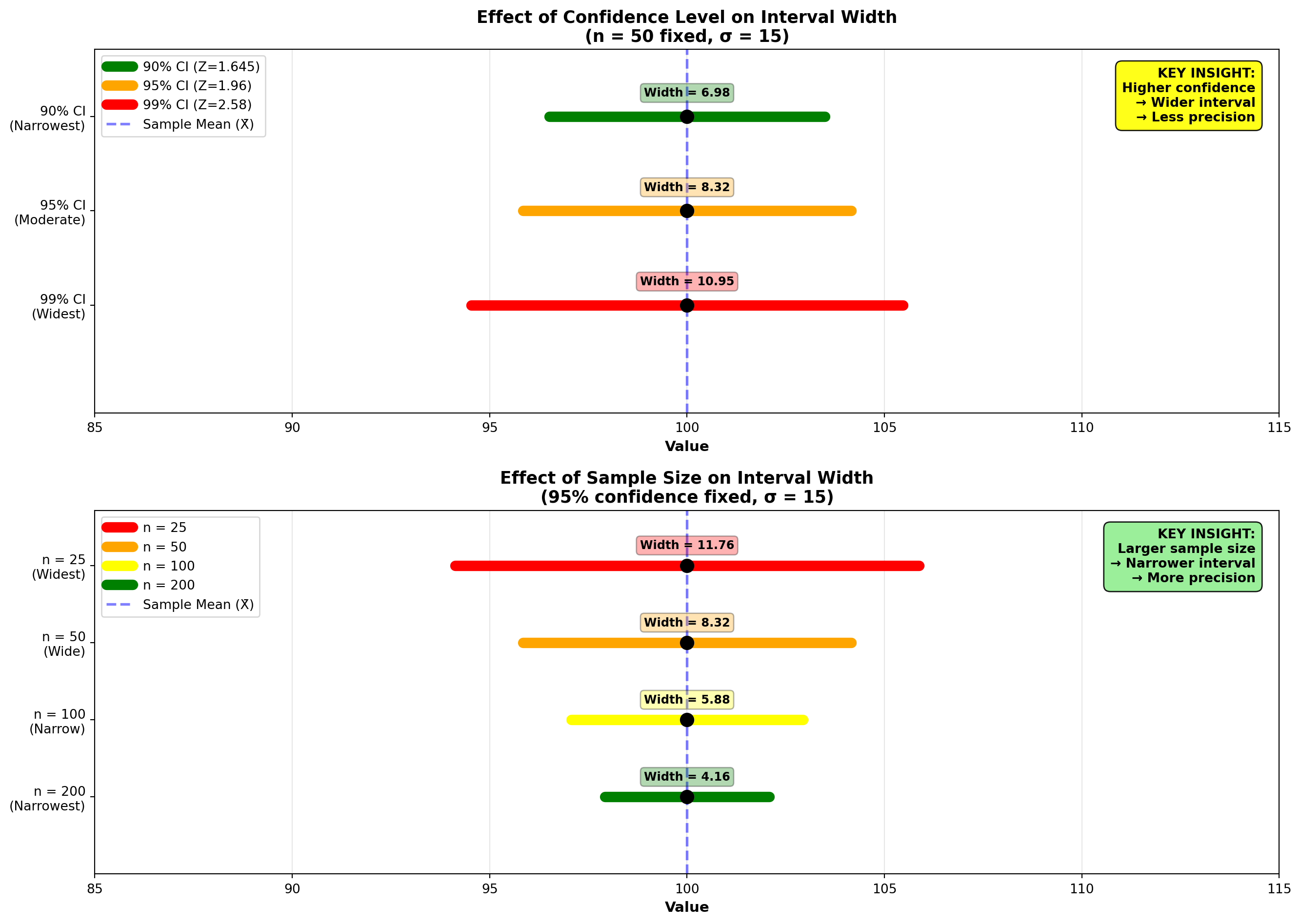
8.7.14 Example 7.10: Comparing Interval Widths
A quality control manager needs to estimate the average diameter of ball bearings with high precision. Initial estimates suggest \sigma = 0.5 mm. The manager has two options:
Option A: Sample 50 bearings with 99% confidence Option B: Sample 50 bearings with 95% confidence
Solution Option A (99% confidence):
\text{Margin of Error} = 2.58 \times \frac{0.5}{\sqrt{50}} = 2.58 \times 0.0707 = 0.182 \text{ mm}
Width: 2 \times 0.182 = 0.364 mm
Solution Option B (95% confidence):
\text{Margin of Error} = 1.96 \times \frac{0.5}{\sqrt{50}} = 1.96 \times 0.0707 = 0.139 \text{ mm}
Width: 2 \times 0.139 = 0.278 mm
Interpretation:
The manager must decide: Is the 0.086 mm reduction in width worth accepting a 4% increase in error probability (from 1% to 5%)?
For precision manufacturing, the answer might be no—maintain 99% confidence and either: - Accept the wider interval, or - Increase the sample size to achieve both precision and confidence
8.8 7.9 Determining the Appropriate Sample Size
Sample size plays an important role in determining both the probability of error and the precision of the estimate. Once the confidence level has been selected, two important factors influence the sample size:
- The variance of the population (\sigma^2)
- The size of the tolerable error the researcher is willing to accept
While the first factor is beyond the researcher’s control (nothing can be done about the population variance), it is possible to limit the size of the error.
8.8.1 Understanding Tolerable Error
The size of error a researcher can tolerate depends on how critical the work is:
- Extremely delicate tasks require exact results:
- Medical procedures on which human lives depend
- Production of machine parts that must meet precise measurements
- Small errors only
- Less critical tasks can accept larger errors with fewer serious consequences
NoteTolerable Error Example
Suppose in manufacturing a part for CD players, an error of 2 millimeters (mm) in the diameter would cause no problem. However, any error greater than 2 mm would result in a defective player.
If a part can vary above and below some desired diameter by 2 mm, this allows an interval of 4 mm. Any given interval is two times the tolerable error.
\text{Interval Width} = 2 \times \text{Tolerable Error}
Therefore: \text{Tolerable Error} = \frac{\text{Interval Width}}{2}
Visual representation:
Code
import matplotlib.pyplot as plt
import numpy as np

fig, ax = plt.subplots(figsize=(12, 6))

# Parameters
target = 50  # mm
error = 2    # mm
lcl = target - error
ucl = target + error

# Draw the acceptable range
ax.fill_between([lcl, ucl], [0, 0], [1, 1], alpha=0.3, color='green',
                label='Acceptable Range')

# Draw the interval boundaries
ax.axvline(lcl, color='red', linestyle='--', linewidth=3, label='LCL = 48 mm')
ax.axvline(target, color='blue', linestyle='-', linewidth=3, label='Target = 50 mm')
ax.axvline(ucl, color='red', linestyle='--', linewidth=3, label='UCL = 52 mm')

# Draw rejection zones
ax.fill_between([45, lcl], [0, 0], [1, 1], alpha=0.2, color='red',
                label='Rejection Zone (Too Small)')
ax.fill_between([ucl, 55], [0, 0], [1, 1], alpha=0.2, color='red',
                label='Rejection Zone (Too Large)')

# Add error arrows
ax.annotate('', xy=(lcl, 0.5), xytext=(target, 0.5),
           arrowprops=dict(arrowstyle='<->', lw=3, color='orange'))
ax.text((lcl + target) / 2, 0.6, 'Error = 2 mm',
       ha='center', fontsize=11, fontweight='bold',
       bbox=dict(boxstyle='round,pad=0.4', facecolor='yellow', alpha=0.9))

ax.annotate('', xy=(ucl, 0.5), xytext=(target, 0.5),
           arrowprops=dict(arrowstyle='<->', lw=3, color='orange'))
ax.text((ucl + target) / 2, 0.6, 'Error = 2 mm',
       ha='center', fontsize=11, fontweight='bold',
       bbox=dict(boxstyle='round,pad=0.4', facecolor='yellow', alpha=0.9))

# Add interval width arrow
ax.annotate('', xy=(ucl, 0.2), xytext=(lcl, 0.2),
           arrowprops=dict(arrowstyle='<->', lw=3, color='darkgreen'))
ax.text(target, 0.1, 'Interval Width = 4 mm\n(2 × Tolerable Error)',
       ha='center', fontsize=11, fontweight='bold',
       bbox=dict(boxstyle='round,pad=0.4', facecolor='lightgreen', alpha=0.9))

# Add value labels
ax.text(lcl, 0.85, f'LCL\n{lcl} mm', ha='center', fontsize=10, fontweight='bold',
       bbox=dict(boxstyle='round,pad=0.3', facecolor='lightcoral', alpha=0.9))
ax.text(target, 0.85, f'Target\n{target} mm', ha='center', fontsize=10, fontweight='bold',
       bbox=dict(boxstyle='round,pad=0.3', facecolor='lightblue', alpha=0.9))
ax.text(ucl, 0.85, f'UCL\n{ucl} mm', ha='center', fontsize=10, fontweight='bold',
       bbox=dict(boxstyle='round,pad=0.3', facecolor='lightcoral', alpha=0.9))

# Formatting
ax.set_title('CD Player Part Manufacturing: Tolerable Error Specification\nDesired Diameter = 50 mm ± 2 mm',
            fontsize=13, fontweight='bold')
ax.set_xlabel('Part Diameter (mm)', fontsize=11, fontweight='bold')
ax.set_ylabel('', fontsize=11)
ax.set_xlim(45, 55)
ax.set_ylim(0, 1)
ax.set_yticks([])
ax.grid(True, alpha=0.3, axis='x')
ax.legend(loc='upper right', fontsize=9, ncol=2)

# Add formula box
formula_text = (
    "KEY FORMULAS:\n"
    "Interval Width = 2 × Error\n"
    "Error = Width / 2\n\n"
    "This Example:\n"
    "Width = 4 mm\n"
    "Error = 2 mm"
)
ax.text(0.02, 0.5, formula_text, transform=ax.transAxes,
       fontsize=9, verticalalignment='center',
       bbox=dict(boxstyle='round,pad=0.5', facecolor='lightyellow', alpha=0.95))

plt.tight_layout()
plt.show()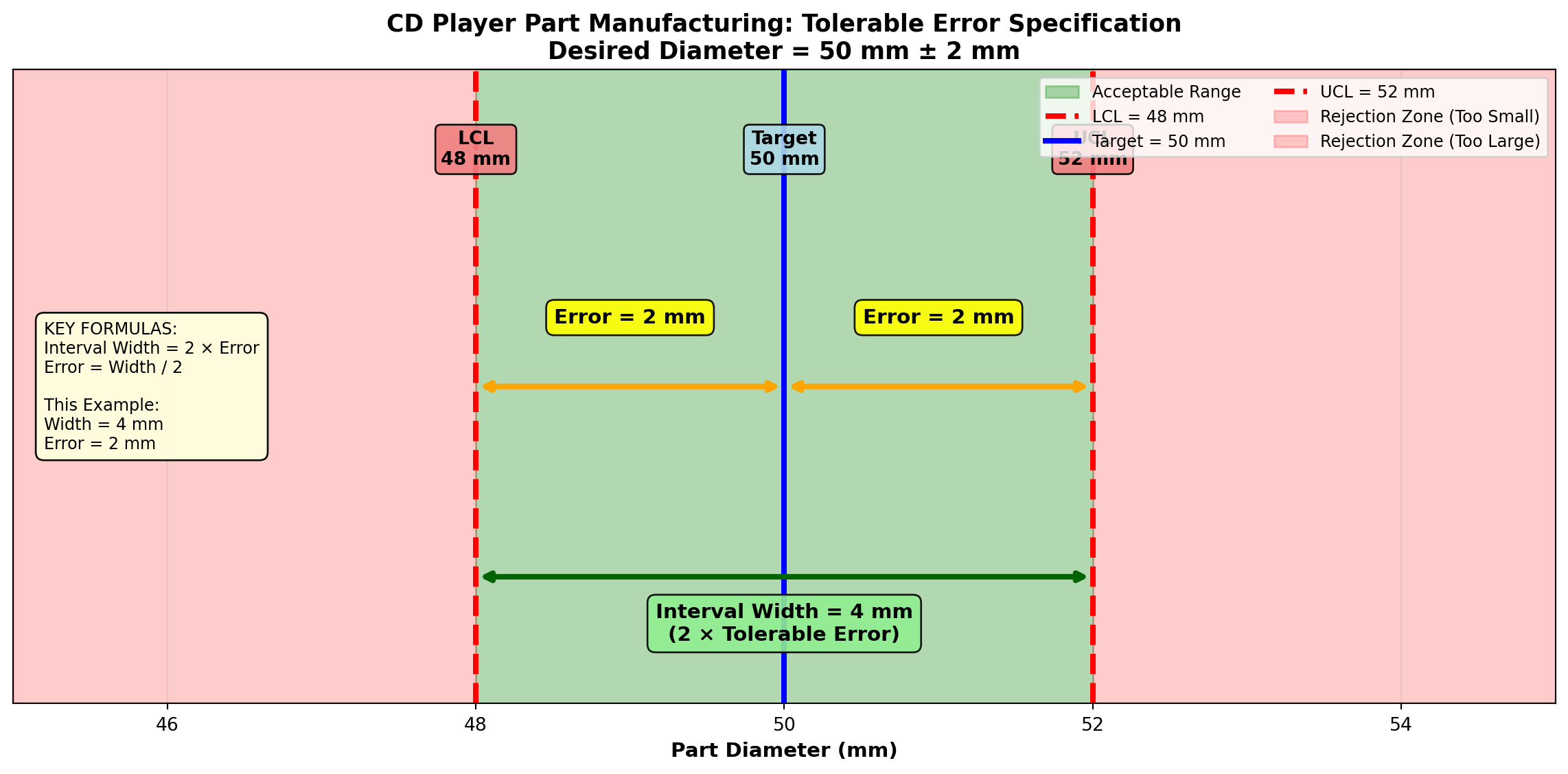
8.8.2 Sample Size for Estimating μ
Recall that the standard normal deviation Z can be expressed as:
Z = \frac{\bar{X} - \mu}{\sigma_{\bar{X}}} = \frac{\bar{X} - \mu}{\sigma/\sqrt{n}}
This can be rewritten algebraically as:
n = \frac{Z^2\sigma^2}{(\bar{X} - \mu)^2} \tag{8.9}
where the difference between the sample mean and the population mean (\bar{X} - \mu) is the error.
In the CD player example above, with a tolerable error of 2 mm, the formula would be written as:
n = \frac{Z^2\sigma^2}{(2)^2} = \frac{Z^2\sigma^2}{4}
8.8.3 Determining Unknown σ
The value of Z depends on the required confidence level. This leaves only \sigma^2 to be determined to calculate the appropriate sample size.
In the likely event that \sigma^2 is unknown, it can be estimated using the sample standard deviation s from a pilot sample of any reasonable size (n \geq 30). The variance calculated from this preliminary sample can then be used in the formula.
8.8.4 Example 7.11: CD Player Manufacturing
The manufacturer of CD players wants to construct a 95% interval for the average size of the part. A pilot sample has revealed a standard deviation of 6 mm. How large should the sample be?
Solution:
A 95% interval gives a Z-value of 1.96. The tolerable error is 2 mm. Therefore:
\begin{aligned} n &= \frac{Z^2\sigma^2}{(\text{error})^2} \\ &= \frac{(1.96)^2(6)^2}{(2)^2} \\ &= \frac{(3.8416)(36)}{4} \\ &= \frac{138.30}{4} \\ &= 34.57 \text{ or } 35 \text{ parts} \end{aligned}
Interpretation:
The manufacturer should select a sample of 35 parts. From this sample, a 95% interval could be constructed for the average size. The interval would have an error no greater than 2 mm.
ImportantRounding Rule for Sample Size
Always round UP to the next whole number, even if the decimal is less than 0.5.
Why? Because rounding down would give you slightly less precision than required. Since you can’t sample a fraction of a unit, rounding up ensures you meet or exceed your precision requirements.
8.8.5 Example 7.12: Wisconsin Ski Resort Snowfall Study
The owner of a ski resort in southern Wisconsin is considering purchasing a snow-making machine to help Mother Nature provide an appropriate base for skiing enthusiasts. If average snowfall seems insufficient, he thinks the machine should pay for itself very soon.
He plans to estimate the average inches of snow that fall in the area, but has no idea how large the sample should be. He only knows that he wants 99% confidence in his findings and that the error must not exceed 1 inch.
Solution:
Begin with a pilot sample (large, n \geq 30) that produces a standard deviation of 3.5 inches. Therefore:
\begin{aligned} n &= \frac{Z^2(s)^2}{(\text{error})^2} \\ &= \frac{(2.58)^2(3.5)^2}{(1)^2} \\ &= \frac{(6.6564)(12.25)}{1} \\ &= 81.54 \text{ or } 82 \text{ snowfalls} \end{aligned}
Interpretation:
The owner should collect data on the last 82 snowfalls during previous years. With this information, he can determine if Mother Nature needs help. Most importantly, you can spend the rest of the winter skiing for free (as promised for helping)!
8.8.6 Sample Size for Estimating π
In Chapter 6 we found that:
Z = \frac{p - \pi}{\sigma_p}
where
\sigma_p = \sqrt{\frac{\pi(1-\pi)}{n}}
We can rewrite this to produce an expression for sample size:
n = \frac{Z^2(\pi)(1-\pi)}{(p - \pi)^2} \tag{8.10}
where (p - \pi) is the difference between the sample proportion and the population proportion, and therefore is the error.
8.8.7 The Problem: π is Unknown
The formula requires the value of \pi. However, \pi is the parameter we want to estimate and is unknown! This problem can be handled in one of two ways:
8.8.7.1 Option 1: Use a Pilot Sample
Take a pilot sample to obtain a preliminary value for \pi, just as we did when determining the appropriate sample size for the mean.
8.8.7.2 Option 2: Use π = 0.5 (Conservative Approach)
Determine that \pi = 0.5 for purposes of determining sample size. This method is often preferred because it is very “safe” or conservative—it guarantees the largest possible sample size given any confidence level and desired error.
Why π = 0.5 gives the largest sample size:
The numerator of the formula contains \pi(1-\pi), which is maximized when \pi = 1 - \pi = 0.5.
If \pi = 0.5, then \pi(1-\pi) = (0.5)(0.5) = 0.25.
No other value of π produces a larger product:
| π | 1-π | π(1-π) | Sample Size |
|---|---|---|---|
| 0.1 | 0.9 | 0.09 | Smaller |
| 0.2 | 0.8 | 0.16 | Smaller |
| 0.3 | 0.7 | 0.21 | Smaller |
| 0.4 | 0.6 | 0.24 | Smaller |
| 0.5 | 0.5 | 0.25 | LARGEST |
| 0.6 | 0.4 | 0.24 | Smaller |
| 0.7 | 0.3 | 0.21 | Smaller |
| 0.8 | 0.2 | 0.16 | Smaller |
| 0.9 | 0.1 | 0.09 | Smaller |
Any value other than 0.5 would result in \pi(1-\pi) < 0.25, and therefore n would be smaller.
8.8.8 Example 7.13: Political Campaign Polling
Wally Simpleton is running for governor. He wants to estimate within 1 percentage point the proportion of people who will vote for him. He also wants to be 95% confident in his findings. How large should the sample size be?
Solution:
Using the conservative approach with \pi = 0.5:
\begin{aligned} n &= \frac{Z^2\pi(1-\pi)}{(\text{error})^2} \\ &= \frac{(1.96)^2(0.5)(0.5)}{(0.01)^2} \\ &= \frac{(3.8416)(0.25)}{0.0001} \\ &= \frac{0.9604}{0.0001} \\ &= 9,604 \text{ voters} \end{aligned}
Interpretation:
A sample of 9,604 voters will allow Wally to estimate \pi with an error of 1% and a confidence level of 95%.
NotePolitical Polling Reality
This explains why professional political polls typically survey 1,000-1,500 people: - For a ±3% margin of error at 95% confidence: n = \frac{(1.96)^2(0.25)}{(0.03)^2} \approx 1,067 - Pollsters balance cost against precision - The 1% error that Wally wants requires nearly 10 times the sample size!
8.8.9 Example 7.14: City Council Smoking Ban
The city council is planning a law prohibiting smoking in public buildings including restaurants, taverns, and theaters. Only private residences will be exempt. Before the law is brought before the council, they want to estimate the proportion of residents who support the plan.
Lacking statistical ability, the council hires you as a consultant. Your first step will be to determine the necessary sample size. You are told that your error must not exceed 2% and you must be 95% sure of your results.
Solution:
Since no pilot survey was previously taken, you must set \pi at 0.5 for purposes of solving for sample size:
\begin{aligned} n &= \frac{Z^2\pi(1-\pi)}{(\text{error})^2} \\ &= \frac{(1.96)^2(0.5)(0.5)}{(0.02)^2} \\ &= \frac{(3.8416)(0.25)}{0.0004} \\ &= \frac{0.9604}{0.0004} \\ &= 2,401 \text{ citizens} \end{aligned}
Interpretation:
With the data supplied by the 2,401 people, you can proceed with your estimate of the proportion of all residents who favor the law. The council can make its determination regarding the city-wide policy on smoking based on solid statistical evidence.
8.8.10 Summary Formulas for Sample Size Determination
ImportantSample Size Formulas
For estimating the population mean μ:
n = \frac{Z^2\sigma^2}{E^2}
where E is the tolerable error (margin of error).
For estimating the population proportion π:
n = \frac{Z^2\pi(1-\pi)}{E^2}
If \pi is unknown, use \pi = 0.5 for a conservative (larger) sample size.
Common Z-values: - 90% confidence: Z = 1.645 - 95% confidence: Z = 1.96 - 99% confidence: Z = 2.58
8.8.11 Quick Reference: Sample Size Trade-offs
graph LR
    A[Sample Size<br/>Decision] --> B[Increase n]
    A --> C[Decrease n]

    B --> B1[✓ Narrower CI<br/>✓ More precision<br/>✗ Higher cost<br/>✗ More time]

    C --> C1[✓ Lower cost<br/>✓ Less time<br/>✗ Wider CI<br/>✗ Less precision]

    style A fill:#FFD700
    style B fill:#90EE90
    style C fill:#FFB6C6
8.9 7.10 Properties of Good Estimators
8.9.1 Estimators vs. Estimates
A distinction must be made between an estimator and an estimate:
- An estimator is the rule or procedure, usually expressed as a formula, used to derive the estimate
- An estimate is the numerical result of the estimator
Example:
\bar{X} = \frac{\sum X_i}{n}
is the estimator for the population mean. If the value of the estimator \bar{X} is, say, 10, then 10 is the estimate of the population mean.
NoteDefinition: Estimators and Estimates
An estimator is the process by which the estimate is obtained.
An estimate is the numerical result of the estimator.
8.9.2 Four Desirable Properties
To perform reliably, estimators should be:
- Unbiased
- Efficient
- Consistent
- Sufficient
Each property is discussed in this section.
8.9.3 Property 1: Unbiased Estimator
As noted in Chapter 6, it is possible to construct a sampling distribution by selecting all possible samples of a given size from a population. An estimator is unbiased if the mean of the statistic calculated in all these samples equals the corresponding parameter.
Let \theta (the Greek letter theta) be the parameter we’re trying to estimate using \hat{\theta} (read “theta hat”). Then \hat{\theta} is an unbiased estimator if its mean, or expected value E(\hat{\theta}), equals \theta. That is:
E(\hat{\theta}) = \theta \tag{8.11}
Example: \bar{X} is an unbiased estimator of \mu because the mean of the sampling distribution of sample means, \bar{\bar{X}}, equals \mu. Therefore:
E(\bar{X}) = \bar{\bar{X}} = \mu
ImportantDefinition: Unbiased Estimator
An estimator is unbiased if the mean of its sampling distribution equals the corresponding parameter.
Visual representation:
Code
import matplotlib.pyplot as plt
import numpy as np
from scipy import stats

fig, axes = plt.subplots(1, 2, figsize=(14, 6))

# True parameter value
theta = 100

# Generate sampling distributions
x = np.linspace(85, 125, 1000)

# Unbiased estimator: centered at theta
unbiased_dist = stats.norm(loc=theta, scale=5)
y_unbiased = unbiased_dist.pdf(x)

# Biased estimator: shifted to the right
biased_dist = stats.norm(loc=110, scale=5)
y_biased = biased_dist.pdf(x)

# Panel 1: Unbiased Estimator
axes[0].plot(x, y_unbiased, 'b-', linewidth=3, label='Sampling Distribution of θ̂₁')
axes[0].fill_between(x, y_unbiased, alpha=0.3, color='blue')

# Mark true parameter and expected value
axes[0].axvline(theta, color='green', linestyle='--', linewidth=3,
                label=f'True θ = {theta}')
axes[0].axvline(theta, color='darkgreen', linestyle='-', linewidth=2, alpha=0.7,
                label=f'E(θ̂₁) = {theta}')

axes[0].set_title('UNBIASED Estimator\nE(θ̂₁) = θ',
                  fontsize=13, fontweight='bold', color='green')
axes[0].set_xlabel('Estimator Value', fontsize=11, fontweight='bold')
axes[0].set_ylabel('Probability Density', fontsize=11, fontweight='bold')
axes[0].legend(loc='upper right', fontsize=10)
axes[0].grid(True, alpha=0.3)
axes[0].set_ylim(0, max(y_unbiased) * 1.15)

# Add annotation
axes[0].annotate('Distribution centered\nat true parameter',
                xy=(theta, max(y_unbiased)/2),
                xytext=(theta - 8, max(y_unbiased) * 0.8),
                arrowprops=dict(arrowstyle='->', lw=2, color='green'),
                fontsize=10, fontweight='bold',
                bbox=dict(boxstyle='round,pad=0.5', facecolor='lightgreen', alpha=0.8))

# Panel 2: Biased Estimator
axes[1].plot(x, y_biased, 'r-', linewidth=3, label='Sampling Distribution of θ̂₂')
axes[1].fill_between(x, y_biased, alpha=0.3, color='red')

# Mark true parameter and biased expected value
axes[1].axvline(theta, color='green', linestyle='--', linewidth=3,
                label=f'True θ = {theta}')
axes[1].axvline(110, color='darkred', linestyle='-', linewidth=2,
                label='E(θ̂₂) = 110')

# Show bias with arrow
axes[1].annotate('', xy=(110, max(y_biased) * 0.4),
                xytext=(theta, max(y_biased) * 0.4),
                arrowprops=dict(arrowstyle='<->', lw=3, color='orange'))
axes[1].text(105, max(y_biased) * 0.5, 'BIAS = +10',
            fontsize=11, fontweight='bold', color='orange',
            bbox=dict(boxstyle='round,pad=0.3', facecolor='yellow', alpha=0.9))

axes[1].set_title('BIASED Estimator (Upward Bias)\nE(θ̂₂) ≠ θ',
                  fontsize=13, fontweight='bold', color='red')
axes[1].set_xlabel('Estimator Value', fontsize=11, fontweight='bold')
axes[1].set_ylabel('Probability Density', fontsize=11, fontweight='bold')
axes[1].legend(loc='upper right', fontsize=10)
axes[1].grid(True, alpha=0.3)
axes[1].set_ylim(0, max(y_biased) * 1.15)

# Add annotation
axes[1].annotate('Distribution shifted\naway from true value',
                xy=(110, max(y_biased)/2),
                xytext=(115, max(y_biased) * 0.8),
                arrowprops=dict(arrowstyle='->', lw=2, color='red'),
                fontsize=10, fontweight='bold',
                bbox=dict(boxstyle='round,pad=0.5', facecolor='lightyellow', alpha=0.8))

plt.tight_layout()
plt.show()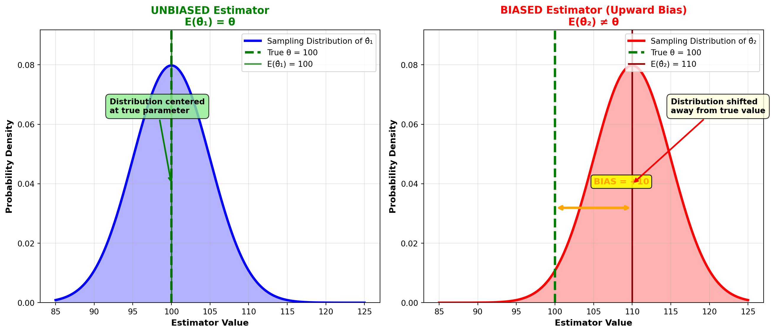
The figure illustrates how the mean of a sampling distribution must equal the corresponding parameter to ensure an unbiased estimator.
Here, \hat{\theta}_1 is an unbiased estimator of \theta because its distribution is centered on \theta. Therefore, E(\hat{\theta}_1) = \theta. If many different samples were taken, producing many different values for \hat{\theta}_1, their mean would equal \theta.
Conversely, if many samples are taken and \hat{\theta}_2 is calculated each time, its mean would exceed \theta. Therefore, \hat{\theta}_2 is a biased estimator (upward bias) of \theta.
Measure of bias:
\text{Bias} = E(\hat{\theta}_2) - \theta
Note that: - E(\hat{\theta}_1) - \theta = 0 (unbiased) - E(\hat{\theta}_2) - \theta \neq 0 (biased)
8.9.4 Property 2: Efficient Estimator
The efficiency of an estimator depends on its variance. Let \hat{\theta}_1 and \hat{\theta}_2 be two unbiased estimators of \theta. Then \hat{\theta}_1 is a more efficient estimator if, in repeated sampling with a given sample size, its variance is less than that of \hat{\theta}_2.
It is logical that an estimator with smaller variance will estimate the parameter more closely.
Visual representation:
Code
import matplotlib.pyplot as plt
import numpy as np
from scipy import stats

fig, ax = plt.subplots(figsize=(12, 7))

# True parameter value
theta = 100

# Generate sampling distributions (both unbiased, different variances)
x = np.linspace(75, 125, 1000)

# Efficient estimator: small variance
efficient_dist = stats.norm(loc=theta, scale=3)
y_efficient = efficient_dist.pdf(x)

# Inefficient estimator: large variance
inefficient_dist = stats.norm(loc=theta, scale=8)
y_inefficient = inefficient_dist.pdf(x)

# Plot both distributions
ax.plot(x, y_efficient, 'b-', linewidth=3, label='θ̂₁: Efficient (small variance)')
ax.fill_between(x, y_efficient, alpha=0.4, color='blue')

ax.plot(x, y_inefficient, 'r-', linewidth=3, label='θ̂₂: Inefficient (large variance)')
ax.fill_between(x, y_inefficient, alpha=0.3, color='red')

# Mark true parameter
ax.axvline(theta, color='green', linestyle='--', linewidth=3,
          label=f'True θ = {theta}\n(Both estimators unbiased)')

# Add variance annotations
ax.annotate('', xy=(theta - 3, max(y_efficient) * 0.6),
           xytext=(theta + 3, max(y_efficient) * 0.6),
           arrowprops=dict(arrowstyle='<->', lw=2, color='blue'))
ax.text(theta, max(y_efficient) * 0.7, 'σ₁² = 9\n(small)',
       fontsize=10, fontweight='bold', color='blue', ha='center',
       bbox=dict(boxstyle='round,pad=0.3', facecolor='lightblue', alpha=0.9))

ax.annotate('', xy=(theta - 8, max(y_inefficient) * 0.85),
           xytext=(theta + 8, max(y_inefficient) * 0.85),
           arrowprops=dict(arrowstyle='<->', lw=2, color='red'))
ax.text(theta, max(y_inefficient) * 0.95, 'σ₂² = 64\n(large)',
       fontsize=10, fontweight='bold', color='red', ha='center',
       bbox=dict(boxstyle='round,pad=0.3', facecolor='lightcoral', alpha=0.9))

# Add title and labels
ax.set_title('Efficiency Comparison: Both Unbiased, Different Variances\nVar(θ̂₁) < Var(θ̂₂) → θ̂₁ is MORE EFFICIENT',
            fontsize=13, fontweight='bold')
ax.set_xlabel('Estimator Value', fontsize=11, fontweight='bold')
ax.set_ylabel('Probability Density', fontsize=11, fontweight='bold')
ax.legend(loc='upper right', fontsize=11)
ax.grid(True, alpha=0.3)

# Add key insight boxes
ax.text(0.02, 0.97,
       'EFFICIENCY:\nSmaller variance means\nestimates cluster more\ntightly around true value',
       transform=ax.transAxes, fontsize=10, fontweight='bold',
       verticalalignment='top',
       bbox=dict(boxstyle='round,pad=0.5', facecolor='lightgreen', alpha=0.9))

ax.text(0.98, 0.97,
       'Both E(θ̂₁) = E(θ̂₂) = θ\n(UNBIASED)\n\nBut Var(θ̂₁) < Var(θ̂₂)\n→ θ̂₁ PREFERRED',
       transform=ax.transAxes, fontsize=10, fontweight='bold',
       verticalalignment='top', horizontalalignment='right',
       bbox=dict(boxstyle='round,pad=0.5', facecolor='yellow', alpha=0.9))

plt.tight_layout()
plt.show()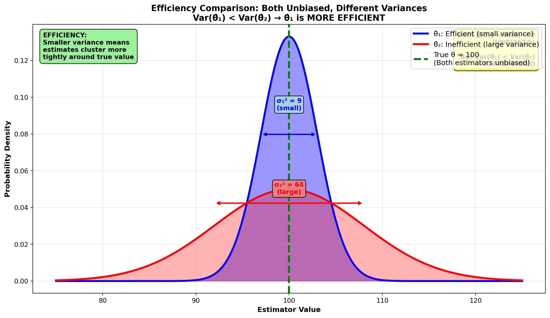
Consider the figure above, which shows the sampling distributions with a given sample size of two statistics \hat{\theta}_1 and \hat{\theta}_2. Both \hat{\theta}_1 and \hat{\theta}_2 are unbiased estimators of \theta because their sampling distributions are centered on \theta, and:
E(\hat{\theta}_1) = E(\hat{\theta}_2) = \theta
However, the variance of the sampling distribution of \hat{\theta}_1 is less than that of \hat{\theta}_2. The possible values for \hat{\theta}_2 are more dispersed. Any estimate of \theta using \hat{\theta}_2 is likely to produce a larger sampling error than an estimate of \theta using \hat{\theta}_1.
ImportantDefinition: Efficient Estimator
Given all unbiased estimators, the most efficient estimator is the one that has the smallest variance.
Example: Among all unbiased estimators of \mu, the sample mean \bar{X} is the most efficient because it has the smallest variance.
8.9.5 Property 3: Consistent Estimator
An estimator is consistent when, as n increases, the estimator approaches the value of the parameter.
ImportantDefinition: Consistent Estimator
An estimator is consistent if, as n increases, the value of the statistic approaches the parameter.
For an estimator to be consistent, it must be unbiased and its variance must approach zero as n increases.
Example: The variance of the sampling distribution of sample means is:
\sigma_{\bar{X}}^2 = \frac{\sigma^2}{n}
As n increases, \sigma_{\bar{X}}^2 approaches zero. Therefore, we can say that \bar{X} is a consistent estimator of \mu.
Visual representation:
Code
import matplotlib.pyplot as plt
import numpy as np
from scipy import stats

fig, axes = plt.subplots(1, 3, figsize=(15, 5))

# True parameter value
mu = 100
sigma = 20  # Population standard deviation

# Different sample sizes
sample_sizes = [10, 50, 200]
colors = ['red', 'orange', 'green']
titles = ['Small Sample (n=10)\nLarge Variance',
          'Medium Sample (n=50)\nModerate Variance',
          'Large Sample (n=200)\nSmall Variance']

x = np.linspace(70, 130, 1000)

for i, (n, color, title) in enumerate(zip(sample_sizes, colors, titles)):
    # Standard error for this sample size
    se = sigma / np.sqrt(n)

    # Sampling distribution
    dist = stats.norm(loc=mu, scale=se)
    y = dist.pdf(x)

    # Plot
    axes[i].plot(x, y, color=color, linewidth=3, label=f'X̄ ~ N(μ, σ²/n)')
    axes[i].fill_between(x, y, alpha=0.4, color=color)

    # Mark true parameter
    axes[i].axvline(mu, color='blue', linestyle='--', linewidth=3,
                   label=f'True μ = {mu}')

    # Mark ±1 SE range
    axes[i].axvline(mu - se, color='gray', linestyle=':', linewidth=2, alpha=0.7)
    axes[i].axvline(mu + se, color='gray', linestyle=':', linewidth=2, alpha=0.7)
    axes[i].fill_between([mu - se, mu + se], [0, 0],
                        [max(y), max(y)], alpha=0.2, color='yellow')

    # Add variance annotation
    axes[i].annotate('', xy=(mu - se, max(y) * 0.5),
                    xytext=(mu + se, max(y) * 0.5),
                    arrowprops=dict(arrowstyle='<->', lw=2, color='black'))
    axes[i].text(mu, max(y) * 0.6, f'σ²/n = {se**2:.2f}\nSE = {se:.2f}',
                fontsize=9, fontweight='bold', ha='center',
                bbox=dict(boxstyle='round,pad=0.3', facecolor='lightyellow', alpha=0.9))

    # Formatting
    axes[i].set_title(title, fontsize=12, fontweight='bold')
    axes[i].set_xlabel('Sample Mean (X̄)', fontsize=10, fontweight='bold')
    axes[i].set_ylabel('Probability Density', fontsize=10, fontweight='bold')
    axes[i].legend(loc='upper right', fontsize=9)
    axes[i].grid(True, alpha=0.3)
    axes[i].set_xlim(70, 130)
    axes[i].set_ylim(0, max(y) * 1.15)

# Add overall title
fig.suptitle('Consistency of X̄: Distribution Becomes More Concentrated as n Increases\nσ²ₓ̄ = σ²/n → 0 as n → ∞',
            fontsize=14, fontweight='bold', y=1.02)

# Add progression arrow
fig.text(0.5, 0.02, '← Increasing Sample Size (n) →',
        ha='center', fontsize=12, fontweight='bold', color='darkgreen',
        bbox=dict(boxstyle='round,pad=0.5', facecolor='lightgreen', alpha=0.8))

plt.tight_layout()
plt.show()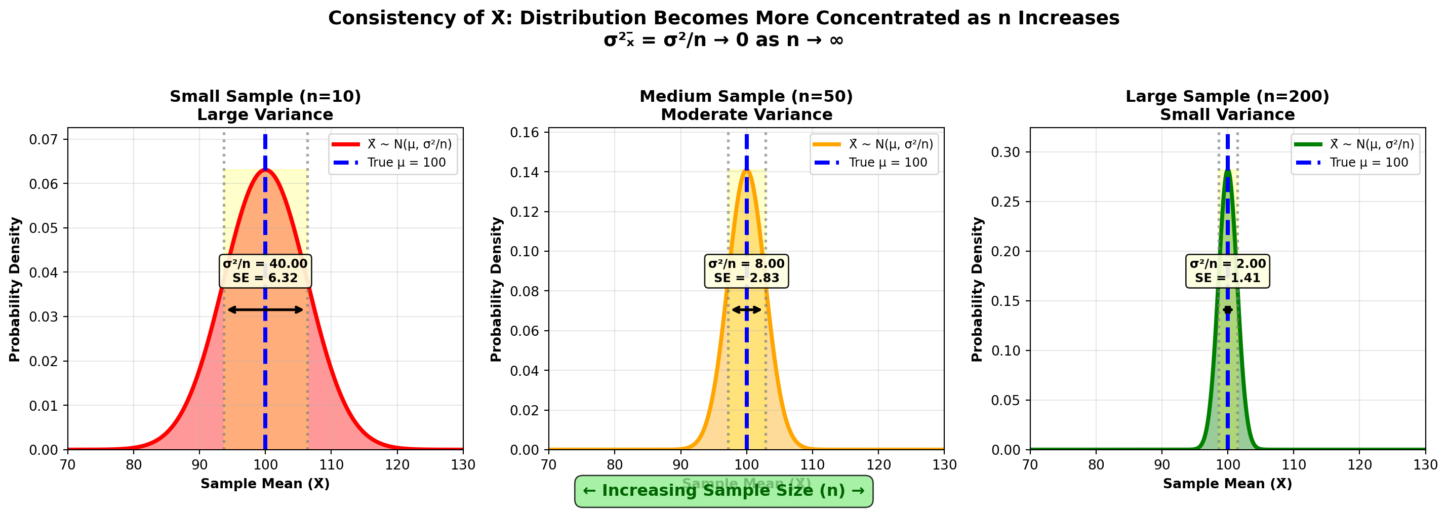
WarningImportance of Consistency
If a statistic is not a consistent estimator, taking a larger sample to improve the estimate will be fruitless. The estimator will not improve with more data.
8.9.6 Property 4: Sufficient Estimator
An estimator is sufficient if it uses all the relevant information about the parameter contained in the sample. If an estimator is sufficient, nothing can be gained by using any other estimator.
ImportantDefinition: Sufficient Estimator
An estimator is sufficient if no other estimator can provide more information about the parameter.
Example: The sample mean \bar{X} is a sufficient estimator for \mu because it uses all n observations in the sample. No other estimator can extract more information about \mu from the same sample.
8.9.7 Summary of Estimator Properties
| Property | Definition | Example |
|---|---|---|
| Unbiased | E(\hat{\theta}) = \theta | E(\bar{X}) = \mu |
| Efficient | Smallest variance among unbiased estimators | \bar{X} has smaller variance than median |
| Consistent | Approaches \theta as n \to \infty | \text{Var}(\bar{X}) = \frac{\sigma^2}{n} \to 0 |
| Sufficient | Uses all relevant information | \bar{X} uses all n observations |
NoteThe “Ideal” Estimator
An ideal estimator possesses all four properties:
- ✓ Unbiased
- ✓ Efficient (minimum variance)
- ✓ Consistent (improves with larger n)
- ✓ Sufficient (uses all information)
The sample mean \bar{X} is an ideal estimator for the population mean \mu because it satisfies all four properties.
8.9.8 Practical Implications
This discussion of estimator properties, while not a complete account, provides a sufficient foundation for evaluating estimation of parameters through the construction of confidence intervals.
Why these properties matter in business:
- Unbiased: Ensures long-run accuracy, no systematic over/under-estimation
- Efficient: Minimizes uncertainty for a given sample size (cost-effective)
- Consistent: Guarantees improvement with more data (scalable)
- Sufficient: Maximizes information extraction (optimal use of resources)
END OF STAGE 3
This completes sections 7.8-7.10 covering: - Controlling interval width through confidence level and sample size - Sample size determination for means and proportions - Properties of good estimators (unbiased, efficient, consistent, sufficient) - Multiple worked examples (CD manufacturing, ski resort, political polling, smoking ban)
Next stage (FINAL) will cover: Problemas Resueltos, Lista de Fórmulas, Chapter Summary, and Closing Scenario. ## Problemas Resueltos {#sec-ci-solved-problems}
This section presents comprehensive worked problems that integrate the concepts covered in this chapter. These problems demonstrate real-world applications of confidence intervals in business decision-making.
8.9.9 Problema Resuelto 1: Artesian Spring Water Distribution
Business Context: Artesian Spring Water provides bottled water in 15-gallon containers to homes in a three-county sector. The manager wants to estimate the average number of containers a typical household uses each month.
A sample of 75 households is taken and the number of containers is recorded. The mean is \bar{X} = 3.2 containers, with s = 0.78 containers.
8.9.9.1 Part (a): 92% Confidence Interval
Question: What would a 92% confidence interval reveal?
Solution:
The Z-value for a 92% confidence interval is found by first dividing 0.92 by 2: thus 0.92/2 = 0.46. An area of 0.46 requires a Z-value of approximately 1.75.
Step 1: Calculate the standard error
s_{\bar{X}} = \frac{s}{\sqrt{n}} = \frac{0.78}{\sqrt{75}} = \frac{0.78}{8.66} = 0.0901 \text{ containers}
Step 2: Find the margin of error
\text{Margin of Error} = Z \times s_{\bar{X}} = 1.75 \times 0.0901 = 0.158 \text{ containers}
Step 3: Construct the confidence interval
\begin{aligned} \text{C.I. for } \mu &= \bar{X} \pm Z s_{\bar{X}} \\ &= 3.2 \pm (1.75)\frac{0.78}{\sqrt{75}} \\ &= 3.2 \pm 0.158 \\ &= 3.042 \leq \mu \leq 3.358 \end{aligned}
Interpretation:
The manager can be 92% confident that the average number of containers used per month by all households is between 3.04 and 3.36 containers.
TipBusiness Decision Insight
This narrow interval (width ≈ 0.32 containers) suggests: - Relatively consistent usage patterns across households - Reliable basis for inventory planning - Can predict demand with reasonable precision at 92% confidence
8.9.9.2 Part (b): Sample Size for Narrower Interval
Question: The manager feels this interval is too wide. How many households must be sampled to be 99% sure that the interval is not wrong by more than 0.10 containers?
Solution:
For a 99% confidence level, Z = 2.58. The tolerable error is 0.10 containers. Using the sample size formula:
\begin{aligned} n &= \frac{Z^2 s^2}{(\text{error})^2} \\ &= \frac{(2.58)^2(0.78)^2}{(0.10)^2} \\ &= \frac{(6.6564)(0.6084)}{0.01} \\ &= \frac{4.0502}{0.01} \\ &= 405.02 \approx 405 \text{ households} \end{aligned}
Interpretation:
A sample of 405 households would yield a 99% confidence interval with an error no greater than 0.10 containers. This represents an 8-fold increase from the original sample (75 → 405) to achieve: - Higher confidence (92% → 99%) - Greater precision (±0.158 → ±0.10)
Cost-benefit analysis: - Benefit: More precise estimate, higher confidence - Cost: 330 additional household surveys needed - Decision: Manager must weigh precision value against data collection costs
8.9.9.3 Part (c): Small Sample for Family Members
Question: A smaller sample of 10 households is selected to estimate the average number of family members per household. The results are: 1, 3, 4, 7, 2, 2, 3, 5, 6, and 6 people. What are the results of a 99% interval for the average number of family members?
Solution:
First, calculate the sample statistics:
\begin{aligned} \bar{X} &= \frac{1+3+4+7+2+2+3+5+6+6}{10} = \frac{39}{10} = 3.9 \text{ people} \\ s &= 1.92 \text{ people (calculated from sample data)} \end{aligned}
Since the sample is small (n = 10 < 30), we must use the t-distribution. With n - 1 = 9 degrees of freedom and a 99% confidence level, from the t-table: t_{0.01,9} = 3.250.
Calculate the confidence interval:
\begin{aligned} \text{C.I. for } \mu &= \bar{X} \pm t s_{\bar{X}} \\ &= 3.9 \pm (3.250)\frac{1.92}{\sqrt{10}} \\ &= 3.9 \pm (3.250)(0.607) \\ &= 3.9 \pm 1.97 \\ &= 1.93 \leq \mu \leq 5.87 \end{aligned}
Interpretation:
We can be 99% confident that the average number of family members per household is between 1.93 and 5.87 people.
WarningNote on Wide Interval
This interval is quite wide (range of nearly 4 people) due to: - Small sample size (n = 10) - High variability in the data (s = 1.92) - High confidence level (99%) - Use of t-distribution (t = 3.250 vs Z = 2.58)
For better precision, a larger sample would be needed.
8.9.9.4 Part (d): Proportion with Water Softeners
Question: Of the 75 households from the original sample, 22 have in-home water softeners. What is the 95% interval estimate of the proportion of all households in the three-county sector that have softeners?
Solution:
The sample proportion is:
p = \frac{22}{75} = 0.2933
Calculate the standard error:
s_p = \sqrt{\frac{p(1-p)}{n}} = \sqrt{\frac{(0.2933)(0.7067)}{75}} = \sqrt{\frac{0.2073}{75}} = \sqrt{0.002764} = 0.0526
Construct the 95% confidence interval (Z = 1.96):
\begin{aligned} \text{C.I. for } \pi &= p \pm Z s_p \\ &= 0.2933 \pm (1.96)(0.0526) \\ &= 0.2933 \pm 0.1031 \\ &= 0.1902 \leq \pi \leq 0.3964 \end{aligned}
Interpretation:
With 95% confidence, between 19.0% and 39.6% of all households in the three-county sector have water softeners.
TipBusiness Application
Artesian Spring Water could use this information to: - Tailor marketing messages about water hardness - Estimate potential market for filtration products - Understand regional water quality perceptions - Plan product offerings based on water softener prevalence
8.9.9.5 Part (e): Narrower Proportion Interval
Question: If an interval ranging from 19.0% to 39.6% of all households having softeners lacks precision, how large a sample must be taken to produce an interval of only 10%?
Solution:
If the confidence interval is to be 10% wide, the tolerable error can only be 5% (since interval width = 2 × error).
Using the conservative approach with \pi = 0.5 for a 95% confidence level:
\begin{aligned} n &= \frac{Z^2\pi(1-\pi)}{(\text{error})^2} \\ &= \frac{(1.96)^2(0.5)(0.5)}{(0.05)^2} \\ &= \frac{(3.8416)(0.25)}{0.0025} \\ &= \frac{0.9604}{0.0025} \\ &= 384.16 \approx 385 \text{ households} \end{aligned}
Interpretation:
A sample of 385 households would be required to estimate the proportion of water softener ownership with: - 95% confidence - Margin of error of ±5% - Total interval width of 10%
This represents a 5-fold increase from the original sample (75 → 385).
8.9.10 Problema Resuelto 2: Investment Industry Returns Analysis
Business Context: An investment analyst wants to estimate the average return for a particular industry sector.
Given: - Population mean return: μ = 30% - Population standard deviation: σ = 12% - Sample size: n = 250 - Question: What is P(\bar{X} > 31%)?
Solution:
This is a sampling distribution problem. Calculate the standard error:
\sigma_{\bar{X}} = \frac{\sigma}{\sqrt{n}} = \frac{12\%}{\sqrt{250}} = \frac{12}{15.81} = 0.759\%
Calculate the Z-score:
Z = \frac{\bar{X} - \mu}{\sigma_{\bar{X}}} = \frac{31 - 30}{0.759} = \frac{1}{0.759} = 1.32
Find the probability:
From the standard normal table, the area from 0 to Z = 1.32 is 0.4066.
Therefore: P(\bar{X} > 31\%) = 0.5 - 0.4066 = 0.0934 = 9.34\%
Interpretation:
There is a 9.34% probability that a random sample of 250 investments from this industry will have an average return exceeding 31%.
NoteInvestment Decision Insight
- If the analyst observes a sample mean > 31%, it’s somewhat unusual (< 10% probability)
- This could indicate the sample is not representative, or
- The industry is performing better than the historical 30% average
- Further investigation would be warranted
8.9.11 Problema Resuelto 3: Direct Marketing Effectiveness
Business Context: A direct marketing firm knows that historically, 22% of recipients respond to their campaigns.
Given: - Population proportion: π = 0.22 - Sample size: n = 250 - Decision rule needed for campaign evaluation
Part (a): Standard Error of the Proportion
\sigma_p = \sqrt{\frac{\pi(1-\pi)}{n}} = \sqrt{\frac{(0.22)(0.78)}{250}} = \sqrt{\frac{0.1716}{250}} = \sqrt{0.0006864} = 0.0262 = 2.62\%
Part (b): Probability of Sample Proportion > 25%
Calculate the Z-score:
Z = \frac{p - \pi}{\sigma_p} = \frac{0.25 - 0.22}{0.0262} = \frac{0.03}{0.0262} = 1.15
From the Z-table, area from 0 to 1.15 is 0.3749.
P(p > 0.25) = 0.5 - 0.3749 = 0.1251 = 12.51\%
Interpretation:
There is a 12.51% probability that a sample of 250 recipients will show a response rate exceeding 25%, even though the true population rate is 22%.
Part (c): 95% Confidence Interval
If the actual sample yields p = 0.25, construct the confidence interval:
s_p = \sqrt{\frac{p(1-p)}{n}} = \sqrt{\frac{(0.25)(0.75)}{250}} = 0.0274
\begin{aligned} \text{C.I. for } \pi &= 0.25 \pm (1.96)(0.0274) \\ &= 0.25 \pm 0.0537 \\ &= 0.1963 \leq \pi \leq 0.3037 \end{aligned}
Business Decision:
Since the historical rate of 22% (0.22) falls within the 95% confidence interval (19.63% to 30.37%), there is insufficient evidence to conclude that the new campaign performs differently from historical norms.
TipMarketing Strategy Implications
- The observed 25% could simply be sampling variation
- No strong evidence of campaign improvement
- Continue monitoring before claiming success
- Consider larger sample for more precise measurement
8.10 Lista de Fórmulas
This comprehensive formula reference organizes all key equations from Chapter 7.
8.10.1 Confidence Intervals for Population Mean (μ)
When σ is known (large samples):
\text{C.I. for } \mu = \bar{X} \pm Z\sigma_{\bar{X}} = \bar{X} \pm Z\frac{\sigma}{\sqrt{n}} \tag{8.12}
When σ is unknown (large samples, n ≥ 30):
\text{C.I. for } \mu = \bar{X} \pm Zs_{\bar{X}} = \bar{X} \pm Z\frac{s}{\sqrt{n}} \tag{8.13}
Small samples (n < 30, population normal, σ unknown):
\text{C.I. for } \mu = \bar{X} \pm ts_{\bar{X}} = \bar{X} \pm t\frac{s}{\sqrt{n}} \tag{8.14}
where t has (n-1) degrees of freedom.
8.10.2 Confidence Intervals for Population Proportion (π)
Standard error of the proportion (population):
\sigma_p = \sqrt{\frac{\pi(1-\pi)}{n}} \tag{8.15}
Estimated standard error (sample):
s_p = \sqrt{\frac{p(1-p)}{n}} \tag{8.16}
Confidence interval for π:
\text{C.I. for } \pi = p \pm Zs_p = p \pm Z\sqrt{\frac{p(1-p)}{n}} \tag{8.17}
8.10.3 Sample Size Determination
For estimating μ:
n = \frac{Z^2\sigma^2}{E^2} \tag{8.18}
where E is the tolerable error (margin of error).
For estimating π:
n = \frac{Z^2\pi(1-\pi)}{E^2} \tag{8.19}
If π is unknown, use \pi = 0.5 (conservative approach).
8.10.4 t-Distribution Properties
Variance of the t-distribution:
\sigma^2 = \frac{n-1}{n-3} \tag{8.20}
Degrees of freedom:
\text{d.f.} = n - 1 \tag{8.21}
8.10.5 Estimator Properties
Unbiased estimator:
E(\hat{\theta}) = \theta \tag{8.22}
Alpha value (probability of error):
\alpha = 1 - \text{Confidence Coefficient} \tag{8.23}
8.10.6 Common Z-values
| Confidence Level | α | α/2 | Z-value |
|---|---|---|---|
| 90% | 0.10 | 0.05 | 1.645 |
| 95% | 0.05 | 0.025 | 1.96 |
| 99% | 0.01 | 0.005 | 2.58 |
8.11 Chapter Summary
This chapter introduced interval estimation as a fundamental tool for making inferences about population parameters under uncertainty.
8.11.1 Key Concepts Mastered
1. Point vs. Interval Estimates - Point estimates provide single values but lack precision measures - Interval estimates provide ranges with associated confidence levels - Confidence intervals quantify uncertainty in estimation
2. Confidence Interval Construction - Structure: Point Estimate ± Margin of Error - Margin of Error = (Critical Value) × (Standard Error) - Confidence level determines the critical value (Z or t)
3. Interpretation of Confidence - Individual interval interpretation: “95% confident this interval contains μ” - Long-run interpretation: “95% of all such intervals will contain μ” - Alpha (α) represents the probability of error
4. Large Sample Confidence Intervals (n ≥ 30) - Use Z-distribution - Standard error: \sigma_{\bar{X}} = \frac{\sigma}{\sqrt{n}} or s_{\bar{X}} = \frac{s}{\sqrt{n}} - Formula: \bar{X} \pm Z \cdot SE
5. Small Sample Confidence Intervals (n < 30) - Requires three conditions: (1) normal population, (2) σ unknown, (3) small n - Use t-distribution with (n-1) degrees of freedom - Formula: \bar{X} \pm t \cdot s_{\bar{X}} - Wider intervals than Z due to additional uncertainty
6. Confidence Intervals for Proportions - Used for binary outcomes (success/failure) - Requires: n\pi > 5 and n(1-\pi) > 5 - Standard error: s_p = \sqrt{\frac{p(1-p)}{n}} - Formula: p \pm Z \cdot s_p
7. Controlling Interval Width - Two methods: (1) Change confidence level, (2) Change sample size - Trade-off: Confidence ↔︎ Precision - Increasing n improves precision without losing confidence
8. Sample Size Determination - For means: n = \frac{Z^2\sigma^2}{E^2} - For proportions: n = \frac{Z^2\pi(1-\pi)}{E^2} - Conservative approach for π: Use 0.5 to maximize sample size - Always round UP to ensure precision requirements are met
9. Properties of Good Estimators - Unbiased: E(\hat{\theta}) = \theta - Efficient: Minimum variance among unbiased estimators - Consistent: Approaches θ as n increases - Sufficient: Uses all available information
8.11.2 Decision Framework
graph TD
    A[Need to estimate<br/>population parameter] --> B{What type<br/>of parameter?}

    B -->|Mean μ| C{What is<br/>sample size?}
    B -->|Proportion π| D[Calculate p = X/n]

    C -->|n ≥ 30| E{Is σ known?}
    C -->|n < 30| F{Is population<br/>normal?}

    E -->|Yes| G[Use Z with σ]
    E -->|No| H[Use Z with s]

    F -->|Yes| I{Is σ known?}
    F -->|No| J[Increase n or use<br/>nonparametric methods]

    I -->|Yes| K[Use Z with σ]
    I -->|No| L[Use t with s]

    D --> M{Is nπ > 5 and<br/>n1-π > 5?}
    M -->|Yes| N[Use Z with sp]
    M -->|No| O[Increase sample size]

    style A fill:#FFD700
    style G fill:#90EE90
    style H fill:#90EE90
    style K fill:#90EE90
    style L fill:#87CEEB
    style N fill:#90EE90
    style J fill:#FFB6C6
    style O fill:#FFB6C6
8.11.3 Critical Business Applications
Throughout this chapter, we’ve seen confidence intervals applied to:
- Quality control: Manufacturing specifications, defect rates
- Finance: Investment returns, portfolio performance
- Marketing: Customer satisfaction, response rates, market share
- Human resources: Employee productivity, turnover rates
- Operations: Service times, inventory levels, capacity utilization
- Public policy: Crime statistics, voter preferences, program effectiveness
8.11.4 The Power of Quantified Uncertainty
Confidence intervals transform business decision-making by:
- Providing actionable ranges rather than point estimates
- Quantifying risk with specific probability levels
- Enabling comparisons across alternatives
- Supporting defensible decisions with statistical evidence
- Communicating uncertainty to stakeholders clearly
8.12 Closing Scenario: FBI Crime Statistics Resolution
Returning to our opening scenario about the FBI’s statistical approach to crime fighting, we can now understand how confidence intervals play a crucial role in criminal profiling and law enforcement strategy.
8.12.1 The FBI Crime Data Analysis
Assume that data were collected for a sample of 1,000 persons who had committed serious crimes. The data reveal that, on average, criminals commit 12.4 illegal acts with a standard deviation of 4.7 before they are arrested or killed.
Question: What proportion of criminals commit more than 15 crimes before capture?
8.12.2 Statistical Analysis
Step 1: Construct a 95% confidence interval for the mean
\begin{aligned} \text{C.I. for } \mu &= \bar{X} \pm Z\frac{s}{\sqrt{n}} \\ &= 12.4 \pm 1.96\frac{4.7}{\sqrt{1000}} \\ &= 12.4 \pm 1.96(0.149) \\ &= 12.4 \pm 0.29 \\ &= 12.11 \leq \mu \leq 12.69 \end{aligned}
Interpretation: The FBI can be 95% confident that the true average number of crimes committed before arrest is between 12.11 and 12.69.
Step 2: Estimate proportion committing > 15 crimes
Using the normal approximation (since n is large):
Z = \frac{X - \mu}{\sigma} = \frac{15 - 12.4}{4.7} = 0.55
From the Z-table: Area from 0 to 0.55 = 0.2088
P(X > 15) = 0.5 - 0.2088 = 0.2912 = 29.12\%
8.12.3 Law Enforcement Implications
ImportantStrategic Insights for Crime Prevention
1. Resource Allocation - Approximately 29% of serious criminals commit more than 15 crimes before capture - Early intervention programs could prevent multiple future crimes - Focus resources on identifying repeat offenders early in their criminal careers
2. Recidivism Patterns - The average of 12.4 crimes provides a benchmark for evaluating intervention effectiveness - Programs showing a reduction below the lower confidence limit (12.11) demonstrate statistical impact - Tracking this metric over time reveals trend in law enforcement effectiveness
3. Predictive Profiling - High standard deviation (4.7) indicates substantial variability in criminal behavior - Some criminals are caught quickly; others evade capture for many crimes - Statistical profiles help predict which suspects pose higher risks
4. Evidence-Based Policy - Confidence intervals provide defensible statistics for budget requests - Policy makers can cite “95% confident” estimates in legislative testimony - Quantified uncertainty supports evidence-based criminal justice reform
8.12.4 The Broader Application
The FBI’s use of confidence intervals demonstrates how statistical inference transforms raw data into actionable intelligence. By quantifying uncertainty:
- Investigators make data-driven decisions about resource deployment
- Administrators justify funding with statistically sound evidence
- Policymakers craft legislation based on empirical patterns
- The public gains confidence in law enforcement effectiveness
This same statistical rigor applies across all business domains: - A retailer estimating customer spending patterns - A manufacturer assessing product quality - A hospital evaluating treatment outcomes - A financial institution measuring portfolio risk
The fundamental principle remains constant: In a world of uncertainty, confidence intervals provide a rigorous framework for making informed decisions with quantified levels of confidence.
8.13 Chapter Exercises
8.13.1 Conceptual Understanding
1. Explain the difference between point estimates and interval estimates. Why are interval estimates generally preferred in business decision-making?
2. If the population mean is unknown, how is it possible to assign a confidence level to an interval estimate? Include a diagram in your answer showing sampling distributions.
3. A 90% interval for estimating the average weight gain of laboratory mice ranges from 0.93 ounces to 1.73 ounces. How would you interpret these results? What Z-value was used in the estimate?
4. Without solving mathematically, explain what would happen to a confidence interval if: a. The confidence level is increased from 95% to 99% b. The sample size is increased from 50 to 200 c. The population standard deviation increases
8.13.2 Confidence Intervals for Means (Large Samples)
5. One hundred 16-ounce cans of Jake’s Mom’s tomato sauce have an average of 15.2 ounces. The population standard deviation in weight is 0.96 ounces. At a 95% confidence level, do the cans appear to be filled with an average of 16 ounces?
6. To estimate average customer spending at the local McDonald’s, statistics students sample 200 customers and find average spending of $5.67 with a standard deviation of $1.10. What is the 95% confidence interval for average spending of all customers? Interpret your results.
7. A study by university professors in Kansas is designed to make inferences about unemployment rates by county in the United States. A sample of 200 counties reports an average rate of 6.2% with a standard deviation of 1.7%. At a 90% confidence level, what is the estimate of the average unemployment rate per county in the nation? Interpret your results.
8. After observing 50 randomly selected television programs, the National Education Association (NEA) reported an average of 32.7 acts of violence in 1997. Assume a sample standard deviation of 10.1. What would your 95% estimate be for the average number of violent acts per program that children see on television?
8.13.3 Confidence Intervals for Means (Small Samples - t-distribution)
9. The Lucky Lady, a popular student hangout, sells 16-ounce glasses of beer. Ten students purchase 22 glasses total, and using their own measuring cup, estimate the average contents. The sample mean is 15.2 ounces with s = 0.86. With a 95% confidence level, do the students believe their money is well spent? Interpret the interval.
10. Dell Publishing samples 23 packages to estimate average postal cost. The sample mean is $23.56 with $s = 4.65. a. The senior editor hopes to keep average cost below $23.00. Calculate and interpret the 99% confidence interval. Will the editor be satisfied? b. Compare results from part (a) with the 99% interval if $s = 2.05. Explain the difference. c. Keeping $s = 4.65, compare part (a) results with the 95% interval. Explain the difference.
11. Bonuses for 10 new National Football League players are used to estimate the average bonus for all new players. The sample mean is $65,890 with $s = 12,300. What is your 90% interval estimate for the population mean?
12. A sample of 25 calls to the Psychic Friends Network reveals an average cost of $23.87. If the standard deviation is $9.56, what is the 98% interval estimate for the average cost of all callers seeking to know their future?
8.13.4 Confidence Intervals for Proportions
13. CNN reported that 68% of all high school students have computers in their homes. If a sample of 1,020 students reveals that 673 have home computers, does a 99% interval support CNN’s claim?
14. In response to the cigarette smoking trend, the National Heart Institute surveyed women to estimate the proportion who smoke occasionally. Of 750 women respondents, 287 said yes. Based on these data, what is your 90% estimate for the proportion of all women who participate in this habit?
15. The National Travel Association sampled people taking vacations in Ireland to estimate how frequently North Americans visit the Emerald Isle. What is the 96% confidence interval for the proportion of tourists who are North American, if 1,098 of the 3,769 surveyed carried U.S. passports?
16. Of the 1,098 North American tourists, 684 had booked their trip through a travel agent. Calculate and interpret the 95% interval for the proportion of all North Americans who use professional travel agency services when visiting Ireland.
8.13.5 Sample Size Determination
17. Days Inn wants to develop a 99% confidence interval to estimate the average number of rooms occupied each night at its nationwide locations. How many nights must be included in the sample if an error of 50 rooms can be tolerated and a pilot sample reveals s = 165 rooms?
18. What would happen to your answer in Exercise 17 if s = 265? Why?
19. How large a sample is required to provide a 90% estimate of the average number of graduates from the nation’s universities with an error of 2,000 students, if a pilot sample reports s = 8,659?
20. A study you’re conducting requires a 95% interval for the average rate of return your company earns on capital budgeting projects. How many projects must your sample include if your supervisor specifies a maximum error of only 5% and s = 2.3\%?
21. As a newly hired employee in the marketing division for a major retail sales concern, you’ve been assigned the task of estimating the proportion of consumers who prefer your product to the competition’s. How many consumers must be sampled if you want to restrict error to 10%, yet provide a 99% confidence level?
22. How large must the sample be in Exercise 21 if error is restricted to 5%? Explain the difference.
23. The credit division of a large commercial bank wants to estimate, with 99% confidence, the proportion of its loans that are delinquent. If the interval width is 7%, how many loans must be reviewed? What is the tolerable error?
8.13.6 Integrated Applications
24. Your product requires that a certain component used in its manufacture average 15.2 grams. If you purchase 100 components and find \bar{X} = 14.8 grams with s = 3.2 grams, what would a confidence interval tell you about the advisability of buying more from this supplier? Your product is very delicate and you feel you can tolerate only a 1% probability of error.
25. If, given the conditions in Exercise 24, the sample had yielded a mean of 14.1 grams, what would you conclude?
26. A textile company found it experiences a total waste factor of 19%. A new process was implemented, and a sample of 1,376 units revealed an average waste factor of 11.1% with a standard deviation of 1.12%. What conclusion can be drawn with a 95% confidence interval about the benefit of the new process?
27. Professional golfers were asked to rate a new graphite club on a scale of 0 to 10. Twenty-five pros generated an average rating of 7.3 with s = 1.01. Construct and interpret the 90% confidence interval.
28. Pizza Pub is considering increasing the price of its large pickle pizza if the average price of its competition exceeds Pizza Pub’s price of $12.95. Thirty-seven other pizzerias report an average price of $12.50 with a standard deviation of 1.01. Pizza Pub wants to be 90% sure of its findings.