11  Analysis of Variance

graph TD
    A[Analysis of Variance] --> B[One-way ANOVA]
    A --> C[Two-way ANOVA]
    A --> D[Factorial Analysis]
    A --> E[Latin Square Design]
    
    B --> B1[How and why<br/>ANOVA works]
    B --> B2[Sums of squares]
    B --> B3[Mean squares]
    B --> B4[The F-ratio]
    B --> F[Pairwise<br/>Comparisons]
    
    C --> C1[The purpose<br/>of blocking]
    C --> C2[Block sums<br/>of squares]
    C --> C3[Two hypothesis<br/>tests]
    
    D --> D1[Interaction]
    D1 --> D2[Hypothesis tests<br/>for interaction]
    
    E --> E1[How it is used<br/>and why]
    E --> E2[Sum of squares<br/>for blocks rows]
    
    F --> F1[Tukey's criterion]
    F --> F2[LSD criterion]
    F --> F3[Common<br/>underlining]
    
    style A fill:#e1f5ff
    style B fill:#fff4e1
    style C fill:#f0fff4
    style D fill:#fff0f5
    style E fill:#f5f0ff

Chapter 10 Conceptual Structure

Opening Scenario: The G-7 Economic Summit

In its June 1997 issue, U.S. News and World Report published a Central Intelligence Agency (CIA) report detailing the economic performance of the world’s largest economies during 1995. The Group of Seven (G-7), called the Summit of Eight since Russia’s inclusion, convened in Denver in 1997 to discuss ways to combat global poverty. Interest focused on the changing state of world economies and the establishment of economic and political policies that would promote global development.

The following table, compiled by the CIA before the G-7 Summit, provides a list of the world’s 10 largest economies with real gross domestic product (GDP).

Rank	Country	GDP (billions US$)	Rank	Country	GDP (billions US$)
1	United States	$7,248	6	France	$1,173
2	China	3,500	7	United Kingdom	1,138
3	Japan	2,679	8	Italy	1,089
4	Germany	1,452	9	Brazil	977
5	India	1,409	10	Russia	796

As several positional changes have occurred among nations over recent years, the Denver discussion centered on the shifting order of the world economy. “A question was raised regarding whether there was any significant downward difference in the sizes of the economies.” G-7 leaders considered that the inflation and unemployment levels listed in the “Closing Scenario” section at the end of this chapter were of special importance in measuring a nation’s economic well-being. The material presented in this chapter will be highly useful in addressing these issues.

Learning Objectives

After studying this chapter and completing the exercises, you will be able to:

1. Understand the logic of analysis of variance and when to apply it
2. Decompose total variation into treatment variation and error variation
3. Calculate sums of squares (total, treatment, and error) for one-way ANOVA
4. Compute mean squares by dividing sums of squares by degrees of freedom
5. Construct and interpret the F-ratio to test equality of population means
6. Use ANOVA tables to summarize and present results professionally
7. Perform post-hoc comparisons using Tukey’s HSD and LSD methods
8. Apply the underlining method to visualize which means differ significantly
9. Distinguish between balanced and unbalanced designs in experimental contexts
10. Make business decisions based on ANOVA results and pairwise comparisons

11.1 10.1 Introduction to Analysis of Variance

In Chapter 9, we tested hypotheses regarding the equality of two population means. Unfortunately, these tests were restricted in their application to a comparison of only two populations. However, many business decisions require comparing more than two populations. This is where analysis of variance (ANOVA) proves invaluable.

NoteWhat is ANOVA?

ANOVA is designed specifically to test whether two or more populations have the same mean. Although the purpose of ANOVA is to test for differences in population means, it involves an examination of sample variances—hence the term analysis of variance.

More specifically, the procedure can be used to determine whether applying a particular “treatment” to a population will have a significant impact on its mean. The use of ANOVA originated in the field of agriculture, where the term treatment was used in the same manner as when treating several plots of land with different fertilizers and noting differences in average crop yields.

Today the term treatment is used broadly, referring to: - Treating customers to different advertising displays and observing differences in average purchases - Treating three groups of employees to three different types of training programs and observing differences in average productivity levels - In general, any situation where a comparison of means is desired

11.1.1 Key ANOVA Terminology

Consider an example measuring the relative effects on employee productivity of three training programs. These three types of training might be: (1) self-directed, (2) computer-based, or (3) supervisor-led.

Experimental Units

The objects that receive the treatment. In our training example, the employees constitute the experimental units.

Factor

The force or variable whose impact on experimental units we wish to measure. In this case, “training” is the factor of interest.

Treatments (or Levels)

The three types of training constitute the treatments, or levels of the factor “training.”

11.1.2 Fixed Effects vs. Random Effects Models

How treatments are selected determines whether we are using a fixed effects model or a random effects model.

Fixed Effects Model

The training program model described above is a fixed effects model. The three training programs were selected or “fixed” before conducting the study. We know which three programs we want to test from the beginning. Conclusions from the study apply only to the three programs included in the study.

Random Effects Model

Suppose Apex Manufacturing had many different training programs available and wanted to know if training programs in general had different effects on employee performance. The three training programs used in the study would be considered a sample of all training programs the firm might use. It doesn’t matter which three methods are used in the study for comparison purposes. Any conclusion from the study is considered applicable to the entire population of training programs.

TipModel Selection

A complete study of random effects models goes beyond the scope of this text. The focus of this chapter will concentrate on fixed effects models, which are most common in business applications.

11.1.3 ANOVA Assumptions

For the application of ANOVA, three assumptions are essential:

1. Normality: All populations involved are normally distributed
2. Homogeneity of variance: All populations have the same variance (\sigma_1^2 = \sigma_2^2 = \cdots = \sigma_c^2)
3. Independence: The samples are selected independently

WarningRobustness of ANOVA

ANOVA is relatively robust to violations of normality and equal variances, especially when sample sizes are equal. However, severe violations can affect the validity of results.

11.1.4 The ANOVA Hypothesis Test

If the number of treatments is designated as c, the hypothesis set for testing is:

\begin{aligned} H_0 &: \mu_1 = \mu_2 = \mu_3 \cdots = \mu_c \\ H_A &: \text{Not all means are equal} \end{aligned}

The letter c is used for the number of treatments because in an ANOVA table (which we’ll see shortly), each treatment is specified in its own column.

11.1.5 Why Not Use Multiple t-Tests?

One might argue that it would be possible to test the equality of several means using various two-sample t-tests, as we did in Chapter 9. However, several complications make this method ineffective.

Example: If a manufacturer wants to compare average daily production for three plants, they could test the three following hypothesis sets:

H_0: \mu_1 = \mu_2 \quad \text{vs.} \quad H_A: \mu_1 \neq \mu_2

H_0: \mu_1 = \mu_3 \quad \text{vs.} \quad H_A: \mu_1 \neq \mu_3

H_0: \mu_2 = \mu_3 \quad \text{vs.} \quad H_A: \mu_2 \neq \mu_3

If the null hypothesis is not rejected in each test, one might conclude that all three means are equal.

Problem 1: Number of Tests

If the number of populations (plants) increases, the number of required tests increases dramatically. With four plants, the number of individual tests doubles from 3 to _4C_2 = 6 tests.

Problem 2: Compounding Alpha

The second and perhaps more troublesome problem arises due to compounding of the \alpha value, which is the probability of a Type I error.

ImportantThe Alpha Inflation Problem

If we conduct three tests at a 5% level, and there are three populations requiring three separate hypothesis tests, the probability of a Type I error exceeds 5%:

\begin{aligned} P(\text{Type I error}) &= [1 - (1-0.05)(1-0.05)(1-0.05)] \\ &= 1 - (0.95)^3 \\ &= 0.1426 \text{ or } 14.26\% \end{aligned}

While we desire to test at a 5% level, the need to conduct three tests increased the probability of Type I error well beyond acceptable limits.

ANOVA solves both problems by testing all means simultaneously in a single test while maintaining the desired significance level.

11.2 10.2 One-Way ANOVA: The Completely Randomized Design

There are several ways in which an ANOVA experiment can be designed. Perhaps the most common is the completely randomized design or one-way ANOVA.

Completely Randomized Design

The term comes from the fact that several subjects or experimental units are randomly assigned to different levels of a single factor. For example, several employees (experimental units) might be randomly selected to participate in various types (different levels) of a training program (the factor).

11.2.1 Business Example: Training Program Effectiveness

The executive director of a large industrial firm wants to determine whether three different training programs have different effects on employee productivity levels. These programs are the treatments that analysis of variance will evaluate.

Fourteen employees are randomly selected and assigned to one of the three programs. Upon completing training, each employee takes an exam to determine their competency. Four employees are placed in the first training program, and five in each of the other two programs. Each of these three groups is treated as independent separate samples.

The test scores appear in Table 10.1, along with some basic calculations.

Table 10.1: Employee Test Scores

	Treatments
	Program 1	Program 2	Program 3
Obs 1	85	80	82
Obs 2	72	84	80
Obs 3	83	81	85
Obs 4	80	78	90
Obs 5	–	82	88
Column means \bar{X}_j	80	81	85

Of the 15 cells in the table, 14 have entries. The last cell of the first treatment is an empty cell. A cell is identified as X_{ij} where i is the row and j is the column in which the cell is located. X_{32} is the entry in the third row and second column: it equals 81. X_{51} is the empty cell.

• The number of rows in each column is indicated with an r
• The number of columns or treatments is indicated with a c
• In the current case, r = 5 and c = 3

As observed in Table 10.1, the mean is calculated for each treatment (column). Because columns are identified by the subscript j, the column averages are represented as \bar{X}_j.

Finally, the grand mean \bar{X} is calculated for all n observations:

\bar{X} = \frac{\sum X_{ij}}{n} = \frac{85 + 72 + 83 + \cdots + 90 + 88}{14} = 82.14

11.2.2 Understanding the Logic of ANOVA

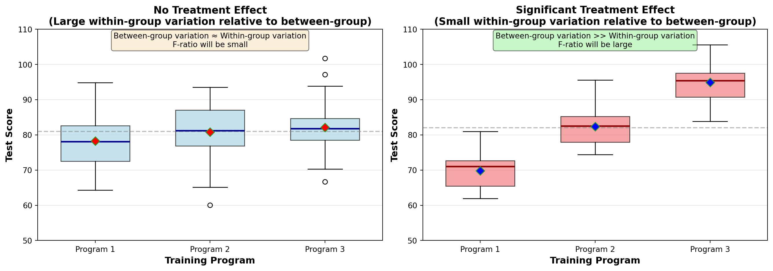
Analysis of variance is based on a comparison of the amount of variation in each of the treatments. If the variation from one treatment to another is significantly high, we can conclude that the treatments have different effects on the populations.

In Table 10.1, we can identify three types or sources of variation. It’s worth noting that the first equals the sum of the other two:

1. Total Variation: There is variation among the total of 14 observations. Not all 14 employees scored the same on the test.

2. Between-Sample Variation: There is variation between the different treatments (samples). Employees in Program 1 did not score the same as those in Programs 2 and 3.

3. Within-Sample Variation: There is variation within a given treatment (sample). Not all employees in the first sample scored the same.

NoteThe Key Insight

By comparing these different sources of variation, we can use analysis of variance to test the equality of population means. Any difference the treatments might have on employee productivity will be detected through a comparison of these forms of variation.

11.3 10.3 How and Why ANOVA Works

To determine whether different treatments have different effects on their respective populations, a comparison is made between within-sample (W/S) variation and between-sample (B/S) variation.

11.3.1 Within-Sample Variation

The variation in scores within a given sample can be produced by a variety of factors: - Innate ability of employees in that sample - Personal motivation - Individual efforts and skill - The luck factor - A host of other random circumstances

Important

The treatment itself will not produce any variation in observations within any sample, because all observations in that sample receive the same treatment.

11.3.2 Between-Sample Variation

It’s a different matter with between-sample variation. The variation in scores between samples (from one sample to the next) can be produced by: - The same random factors as within-sample variation (motivation, skill, luck, etc.) - Plus any additional influence that different treatments might have

Treatment Effect

Because different samples have different treatments, between-sample variation can be produced by the effects of different treatments. This is called the treatment effect.

Figure 11.1: The Logic of ANOVA: Decomposing Variation

NoteDetecting Treatment Effects

If a treatment effect exists, it can be detected by comparing between-sample variation and within-sample variation. If between-sample variation is significantly greater than within-sample variation, a strong treatment effect is present.

This difference between between-sample variation and within-sample variation is precisely what analysis of variance measures.

11.3.3 The F-Ratio in ANOVA Context

The F-Ratio for ANOVA

The F-ratio is a ratio of between-sample variation and within-sample variation.

F = \frac{\text{Between-sample variation}}{\text{Within-sample variation}} = \frac{\text{Treatment variation + Random error}}{\text{Random error}}

Remember: - Between-sample variation can be produced in part by different treatments - Within-sample variation can be produced only by random factors like luck, skill, and employee motivation - This variation is independent of treatment (since all observations within a sample have the same treatment) and results only from random sampling error within the sample

ImportantThe F-Ratio Logic

When population means are different, the treatment effect is present and between-sample deviations will be large compared to error deviation within a sample. Therefore, the F-value will increase, as it is a ratio of treatment variation and error variation.

Total variation equals variation produced by different treatments, plus variation produced by random error elements within treatments such as skill, luck, and motivation:

\text{Total Variation} = \text{Treatment Variation} + \text{Error Variation}

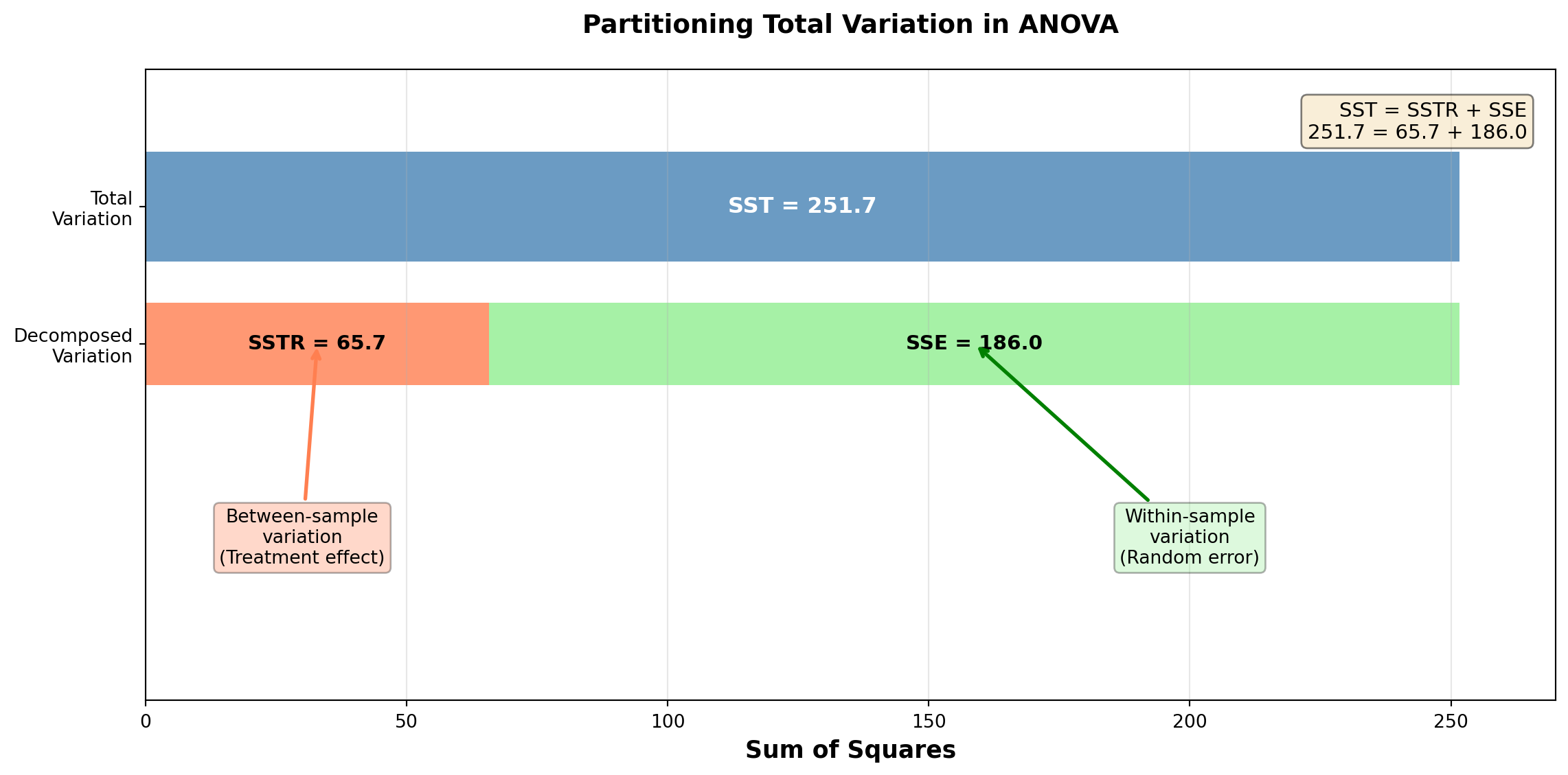
11.4 10.4 Sums of Squares: Partitioning the Variation

Recognition of these three sources of variation allows the partition of the sum of squares, a procedure necessary for analysis of variance. Each of the three types of variation produces a sum of squares:

1. Sum of Squares Total (SST): Measures total variation
2. Sum of Squares Treatment (SSTR): Measures between-sample variation
3. Sum of Squares Error (SSE): Measures within-sample variation

As expected:

SST = SSTR + SSE

This illustrates that SST can be divided into its two components: SSTR and SSE.

11.4.1 Recall: Variance and Sum of Squares

Recall from Chapter 3 that sample variance is calculated as:

s^2 = \frac{\sum(X_i - \bar{X})^2}{n-1}

The numerator is the sum of squared deviations from the mean. Thus, sum of squares is used to measure variation. The denominator is the number of degrees of freedom. This equation serves as a pattern that can be applied to sums of squares in analysis of variance.

11.4.2 Calculating the Sums of Squares

Let X_{ij} be the i-th observation in the j-th sample. For example, X_{21} is the second observation in the first sample. In Table 10.1: - X_{21} = 72 - X_{32} = 81 - X_{43} = 90

Sum of Squares Total (SST)

SST = \sum_{i=1}^{r} \sum_{j=1}^{c} (X_{ij} - \bar{X})^2 \quad [10.3]

The grand mean is subtracted from each of the 14 observations. The differences are squared and summed. The double summation sign indicates this is done across all rows and all columns.

Using data from Table 10.1:

\begin{aligned} SST &= (85 - 82.14)^2 + (72 - 82.14)^2 + (83 - 82.14)^2 + (80 - 82.14)^2 \\ &\quad + (80 - 82.14)^2 + (84 - 82.14)^2 + \cdots + (90 - 82.14)^2 + (88 - 82.14)^2 \\ &= 251.7 \end{aligned}

Note

SST is simply the variation of observations around the grand mean.

Sum of Squares Treatment (SSTR)

SSTR = \sum r_j(\bar{X}_j - \bar{X})^2 \quad [10.4]

The number of observations or rows in each treatment, r_j, is multiplied by the squared differences between each treatment mean, \bar{X}_j, and the grand mean. Results are summed for all treatments.

Formula (10.4) asks that we multiply the number of rows in the j-th column (remember that j denotes a column) by the squared deviation of that column’s mean from the grand mean.

From Table 10.1:

\begin{aligned} SSTR &= 4(80 - 82.14)^2 + 5(81 - 82.14)^2 + 5(85 - 82.14)^2 \\ &= 65.7 \end{aligned}

Note

SSTR reflects the variation in column means around the grand mean.

Sum of Squares Error (SSE)

SSE = \sum \sum (X_{ij} - \bar{X}_j)^2 \quad [10.5]

The treatment mean, \bar{X}_j, is subtracted from each observation in that treatment. The differences are squared and summed. This is done for all treatments, and the results are summed.

Using data from Table 10.1:

\begin{aligned} SSE &= (85-80)^2 + (72-80)^2 + (83-80)^2 + (80-80)^2 \quad \text{(First treatment)} \\ &\quad + (80-81)^2 + (84-81)^2 + (81-81)^2 + (78-81)^2 + (82-81)^2 \quad \text{(Second treatment)} \\ &\quad + (82-85)^2 + (80-85)^2 + (85-85)^2 + (90-85)^2 + (88-85)^2 \quad \text{(Third treatment)} \\ &= 186.0 \end{aligned}

Note

SSE measures random variation of values within a treatment around their own mean.

11.4.3 Verification

A quick review of all these calculations can be made:

SST = SSTR + SSE 251.7 = 65.7 + 186.0 \quad \checkmark

If we trust our arithmetic, we can find SSE simply as:

SSE = SST - SSTR = 251.7 - 65.7 = 186.0

Figure 11.2: Variance Decomposition in One-Way ANOVA

11.5 Section Exercises

Exercise 11.1 (Understanding ANOVA Concepts)  

1. Explain in your own words why ANOVA is preferable to conducting multiple t-tests when comparing more than two population means.

2. What is meant by a “treatment effect” in ANOVA? Provide a business example not mentioned in the text.

3. Calculate the probability of making at least one Type I error when conducting five pairwise t-tests at \alpha = 0.05.

4. Describe the three assumptions required for valid ANOVA results. Which assumption is most critical?

Exercise 11.2 (Sum of Squares Calculation) A company wants to compare customer satisfaction scores across three retail locations. Five customers were surveyed at each location with the following scores (out of 100):

Customer	Location A	Location B	Location C
1	85	78	92
2	88	82	95
3	82	75	88
4	90	80	93
5	85	85	92

Calculate: a. The grand mean \bar{X} b. The column means \bar{X}_j for each location c. SST (Sum of Squares Total) d. SSTR (Sum of Squares Treatment) e. SSE (Sum of Squares Error) f. Verify that SST = SSTR + SSE

11.6 10.5 Mean Squares and Degrees of Freedom

As Formula (10.2) from Chapter 3 indicates for variance, after obtaining the sum of squares, each is divided by its degrees of freedom. A sum of squares divided by its degrees of freedom produces a mean square. That is, if we divide a sum of squares by its degrees of freedom, we obtain a mean square.

NoteDegrees of Freedom Concept

Recall from Chapter 7 that we defined degrees of freedom as the total number of observations in the data set minus any “restrictions” that may be applied. A restriction was any value calculated from the data set.

11.6.1 Degrees of Freedom for Each Sum of Squares

For SST (Total)

In calculating SST, we used the entire data set of n observations to calculate one value. That single value was the grand mean \bar{X}, which represents a restriction. Therefore, SST has n-1 degrees of freedom.

For SSTR (Treatment)

The calculation of SSTR involves the use of c = 3 sample means from which the grand mean can be calculated. The sample means are thus seen as individual data points, and the grand mean is taken as a restriction. SSTR then has c-1 degrees of freedom.

For SSE (Error)

Finally, we calculated SSE earlier by summing the deviation of n = 14 observations from c = 3 sample means. Therefore, SSE has n-c degrees of freedom.

We note that:

\text{d.f. for SST} = \text{d.f. for SSTR} + \text{d.f. for SSE} n - 1 = (c - 1) + (n - c)

11.6.2 Calculating Mean Squares

As noted earlier, because a sum of squares divided by its degrees of freedom produces a mean square, we find the mean square total, or total mean square, CMT:

Total Mean Square

CMT = \frac{SST}{n-1} \quad [10.6]

The treatment mean square (CMTR) is:

Treatment Mean Square

CMTR = \frac{SSTR}{c-1} \quad [10.7]

And the error mean square (CME) is:

Error Mean Square

CME = \frac{SSE}{n-c} \quad [10.8]

11.6.3 Example Calculation: Training Program Data

Using the data from Table 10.1:

\begin{aligned} CMT &= \frac{SST}{n-1} = \frac{251.7}{14-1} = \frac{251.7}{13} = 19.4 \\[10pt] CMTR &= \frac{SSTR}{c-1} = \frac{65.7}{3-1} = \frac{65.7}{2} = 32.9 \\[10pt] CME &= \frac{SSE}{n-c} = \frac{186.0}{14-3} = \frac{186.0}{11} = 16.9 \end{aligned}

ImportantMean Squares are Variances

These three mean squares are modeled from Formula (10.2) for variance. They are sums of squares divided by their degrees of freedom, and as such, they are variances.

11.7 10.6 The F-Ratio for Testing Hypotheses

It is the ratio of the last two mean squares, CMTR and CME, that is used as the basis of analysis of variance to test the hypothesis regarding equality of means. As observed earlier, this ratio conforms to the F distribution and is expressed as:

F-Ratio for Testing Means

F = \frac{CMTR}{CME} \quad [10.9]

In our current case:

F = \frac{32.9}{16.9} = 1.94

NoteInterpreting the F-Ratio

CMTR measures variation between treatments. If treatments have different effects, CMTR will reflect this through its increase. Then, the F-ratio itself will increase.

Therefore, if the F-ratio becomes “significantly” large because CMTR exceeds CME by a large amount, we recognize that treatment effects probably exist. It is likely that different treatments have different effects on the means of their respective populations, and we could reject the null hypothesis \mu_1 = \mu_2 = \mu_3.

11.7.1 Finding the Critical F-Value

The critical value of F that is considered significantly large can be found in Table G (Appendix III) as before. Assume the CEO wants to test the following hypotheses at the 5% level:

\begin{aligned} H_0 &: \mu_1 = \mu_2 = \mu_3 \\ H_A &: \text{Not all means are equal} \end{aligned}

Because CMTR has c - 1 = 3 - 1 = 2 degrees of freedom and CME has n - c = 14 - 3 = 11 degrees of freedom, the critical F-value obtained from the table is:

F_{0.05, 2, 11} = 3.98

The 2 is listed before the 11 when establishing degrees of freedom because CMTR is in the numerator.

Figure 11.3: F-Distribution and Decision Rule for Training Program Example

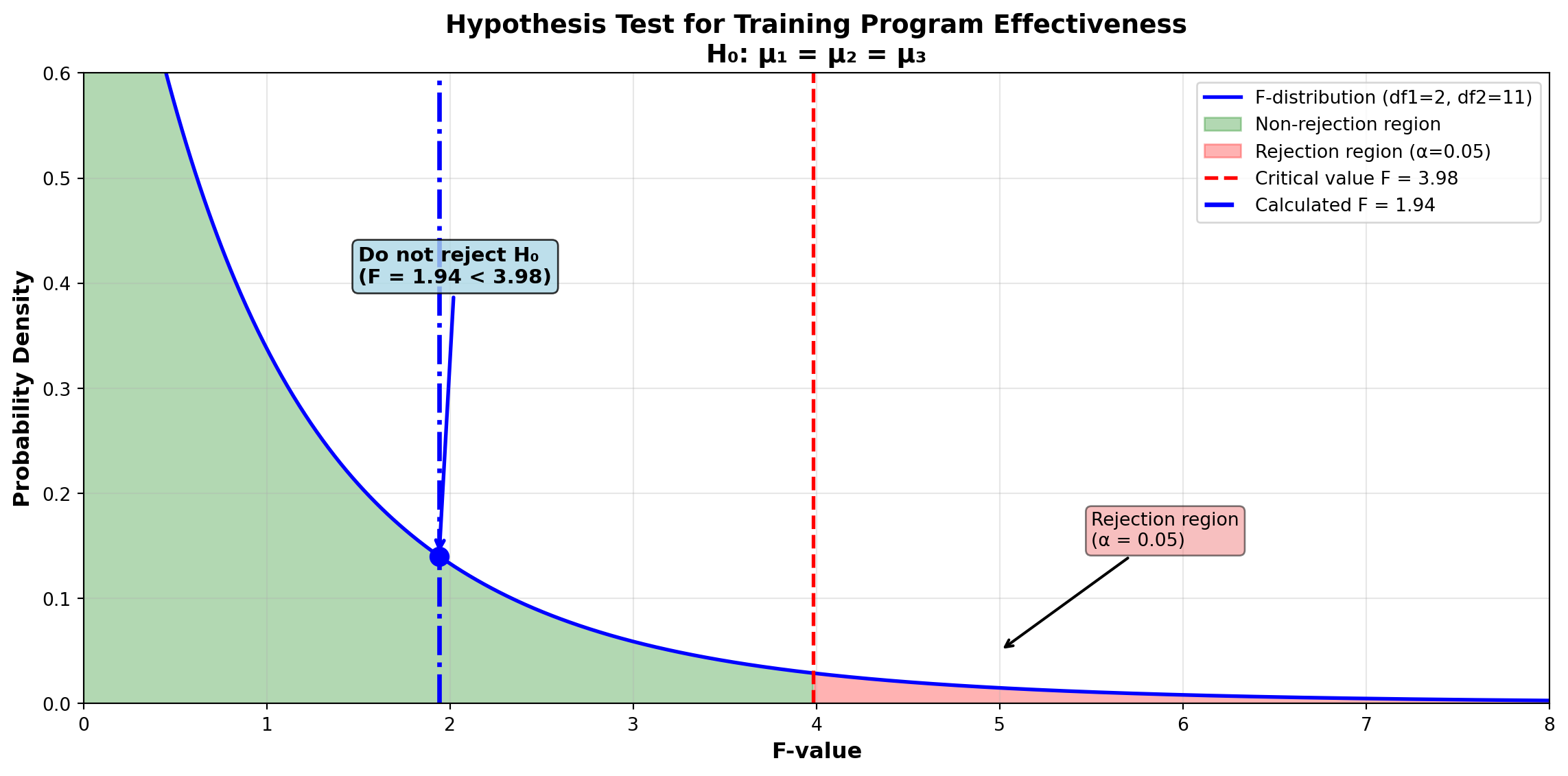
Decision Rule: “Do not reject if F \leq 3.98. Reject the null hypothesis if F > 3.98.”

Because the calculated F-value is 1.94 < 3.98, the CEO should not reject the null hypothesis. They cannot reject at the 5% level the hypothesis that average test scores are the same for all three training programs. There is no significant treatment effect related to any of the programs.

11.8 10.7 The ANOVA Table

It is customary to summarize analysis of variance calculations in a table. The general format of the ANOVA table appears in Table 10.2A, while Table 10.2B contains the specific values from the training program example.

Table 10.2A: General ANOVA Table Format

Source of Variation	Sum of Squares	Degrees of Freedom	Mean Square	F-Value
Between samples (Treatment)	SSTR	c-1	SSTR/(c-1)	CMTR/CME
Within samples (Error)	SSE	n-c	SSE/(n-c)
Total Variation	SST	n-1

Table 10.2B: ANOVA Table for Employee Training Programs

Source of Variation	Sum of Squares	Degrees of Freedom	Mean Square	F-Value
Between samples (Treatment)	65.7	2	32.9	1.94
Within samples (Error)	186.0	11	16.9
Total Variation	251.7	13

Hypotheses: - H_0: \mu_1 = \mu_2 = \mu_3 - H_A: Not all means are equal

Decision Rule: Do not reject if F \leq 3.98. Reject if F > 3.98.

Conclusion: Since F = 1.94 < 3.98, do not reject the null hypothesis.

Note

Note that the relevant sources of variation are listed, and the F-value of 1.94 is shown in the far right column.

11.9 Example 10.1: First City Bank Deposit Analysis

Robert Shade is vice president of marketing at First City Bank in Atlanta. Recent promotional efforts to attract new depositors include games and prizes at four branch locations. Shade is convinced that different types of prizes would attract different income groups. People at one income level prefer gifts, while those at another income group may be more attracted by free trips to favorite vacation spots.

Shade decides to use the amount of deposits as a representative measure of income. He wants to determine if there is a difference in the average deposit level between the four branches. If any difference is found, Shade will offer a variety of promotional prizes.

11.9.1 Solution

Here are seven deposits randomly selected from each branch, rounded to the nearest $100. There are c = 4 treatments (samples) and r_j = 7 observations in each treatment. The total number of observations is n = cr = 28.

Deposit Data (in thousands of dollars)

Deposit	Branch 1	Branch 2	Branch 3	Branch 4
1	5.1	1.9	3.6	1.3
2	4.9	1.9	4.2	1.5
3	5.6	2.1	4.5	0.9
4	4.8	2.4	4.8	1.0
5	3.8	2.1	3.9	1.9
6	5.1	3.1	4.1	1.5
7	4.8	2.5	5.1	2.1
\bar{X}_j	4.87	2.29	4.31	1.46

The grand mean is:

\bar{X} = \frac{\sum X_{ij}}{n} = \frac{5.1 + 4.9 + 5.6 + \cdots + 2.1}{28} = 3.23

Shade wants to test the hypothesis at the 5% level that:

\begin{aligned} H_0 &: \mu_1 = \mu_2 = \mu_3 = \mu_4 \\ H_A &: \text{Not all means are equal} \end{aligned}

11.9.2 Calculations

Using Formulas (10.3) through (10.5):

Sum of Squares Total:

\begin{aligned} SST &= \sum \sum (X_{ij} - \bar{X})^2 \\ &= (5.1 - 3.23)^2 + (4.9 - 3.23)^2 + (5.6 - 3.23)^2 + \cdots + (2.1 - 3.23)^2 \\ &= 61.00 \end{aligned}

Sum of Squares Treatment:

\begin{aligned} SSTR &= \sum r_j(\bar{X}_j - \bar{X})^2 \\ &= 7(4.87 - 3.23)^2 + 7(2.29 - 3.23)^2 + 7(4.31 - 3.23)^2 + 7(1.46 - 3.23)^2 \\ &= 55.33 \end{aligned}

Sum of Squares Error:

\begin{aligned} SSE &= \sum \sum (X_{ij} - \bar{X}_j)^2 \\ &= (5.1 - 4.87)^2 + \cdots + (4.8 - 4.87)^2 \quad \text{(First treatment)} \\ &\quad + (1.9 - 2.29)^2 + \cdots + (2.5 - 2.29)^2 \quad \text{(Second treatment)} \\ &\quad + (3.6 - 4.31)^2 + \cdots + (5.1 - 4.31)^2 \quad \text{(Third treatment)} \\ &\quad + (1.3 - 1.46)^2 + \cdots + (2.1 - 1.46)^2 \quad \text{(Fourth treatment)} \\ &= 5.67 \end{aligned}

Mean Squares:

Formulas (10.7) and (10.8) for mean squares give:

\begin{aligned} CMTR &= \frac{SSTR}{c-1} = \frac{55.33}{3} = 18.44 \\[10pt] CME &= \frac{SSE}{n-c} = \frac{5.67}{24} = 0.236 \end{aligned}

F-Ratio:

F = \frac{CMTR}{CME} = \frac{18.44}{0.236} = 78.14

11.9.3 ANOVA Table and Hypothesis Test

Shade must use 3 and 24 degrees of freedom, since d.f. for SSTR = 3 and d.f. for SSE = 24. If he wants an \alpha of 5%, he finds from Table G (Appendix III) that F_{0.05, 3, 24} = 3.01.

ANOVA Summary Table

Source of Variation	Sum of Squares	Degrees of Freedom	Mean Square	F-Value
Between samples (Treatment)	55.33	3	18.44	78.14
Within samples (Error)	5.67	24	0.236
Total Variation	61.00	27

Hypotheses: - H_0: \mu_1 = \mu_2 = \mu_3 = \mu_4 - H_A: Not all means are equal

Decision Rule: Do not reject if F \leq 3.01. Reject if F > 3.01.

Conclusion: Because F = 78.14 > 3.01, reject the null hypothesis.

C:\Users\patod\AppData\Local\Temp\ipykernel_5344\1940184440.py:19: MatplotlibDeprecationWarning: The 'labels' parameter of boxplot() has been renamed 'tick_labels' since Matplotlib 3.9; support for the old name will be dropped in 3.11.
  bp = ax1.boxplot(data_list, labels=branches, patch_artist=True, showmeans=True,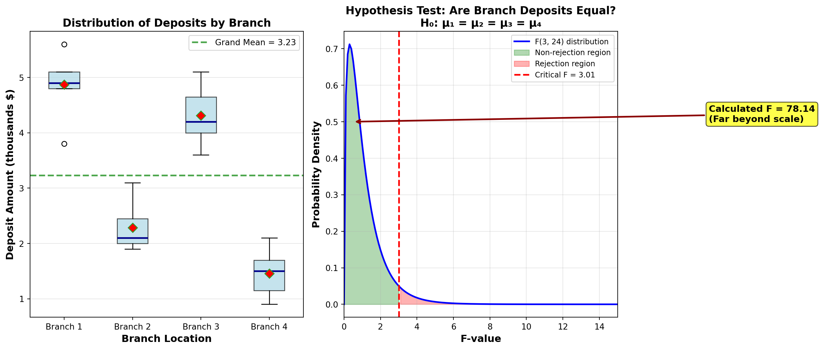

Figure 11.4: Deposit Levels Across Four Bank Branches

11.9.4 Interpretation

Because F = 78.14 (which is extremely large compared to the critical value of 3.01), Shade must reject the null hypothesis. He can be 95% confident that average deposits at all branches are not equal. If he considers that different income groups are attracted by different types of promotional games, he should design alternative schemes for each branch to attract new depositors.

ImportantBusiness Insight

The extremely high F-value (78.14) indicates very strong evidence of differences between branches. This suggests:

1. Customer demographics differ significantly across branch locations
2. Targeted marketing strategies are essential for each branch
3. One-size-fits-all promotions would be ineffective
4. Further analysis (post-hoc tests) is needed to determine which specific branches differ

11.10 Section Exercises

Exercise 11.3 (Constructing ANOVA Tables)  

1. Complete the following ANOVA table and test the hypothesis at \alpha = 0.05 that all population means are equal:

Source of Variation	Sum of Squares	Degrees of Freedom	Mean Square	F-Value
Between samples	450.5	4	?	?
Within samples	892.3	45	?
Total	?	?

2. Given: c = 5 treatments, n = 35 total observations, SST = 1,250, SSTR = 380
   1. Construct a complete ANOVA table
   2. Test at \alpha = 0.01 whether all means are equal
   3. Calculate the p-value for this test

Exercise 11.4 (Production Method Comparison) A manufacturing company wants to compare the output of four different production methods. Random samples of workers using each method yielded the following daily production units:

Method A: 45, 42, 48, 51, 46, 43
Method B: 52, 55, 50, 54, 53
Method C: 38, 41, 39, 42, 40, 37
Method D: 48, 46, 49, 47, 50, 48, 45

1. Calculate the grand mean and treatment means
2. Compute SST, SSTR, and SSE
3. Construct a complete ANOVA table
4. At \alpha = 0.05, test whether average production differs among methods
5. What is your recommendation to management?

Exercise 11.5 (Critical Thinking About ANOVA)  

1. Explain why an F-ratio close to 1.0 suggests no treatment effect exists.

2. What happens to the F-ratio when:

   • Between-sample variation increases while within-sample variation stays constant?
   • Within-sample variation increases while between-sample variation stays constant?

3. Describe a business scenario where ANOVA would be more appropriate than conducting multiple t-tests.

4. Why must the F-distribution be used instead of the normal or t-distribution for ANOVA tests?

11.11 10.8 Post-Hoc Tests: Pairwise Comparisons

As you can observe from the previous explanation, analysis of variance tells us whether all means are equal. However, when we reject the null hypothesis, ANOVA does not reveal which mean(s) differ from the rest. We must use other statistical tests to make this determination.

These tests consist of a pairwise comparison of all possible pairs of means. If the absolute value (ignoring signs) of the difference between any two sample means is greater than some standard, it is observed as a significant difference, and we conclude that the respective population means are different.

NotePurpose of Post-Hoc Tests

Post-hoc (meaning “after this”) tests are performed only after rejecting the null hypothesis in ANOVA. They help us identify: - Which specific groups differ from each other - The magnitude of differences - Patterns of similarity among treatments

This standard can be determined through a variety of statistical procedures, including: - Tukey’s method (also called Tukey’s Honestly Significant Difference or HSD) - Least Significant Difference (LSD) method - Scheffé’s method (for more complex comparisons) - Bonferroni method (controlling family-wise error rate)

We will focus on the most commonly used: Tukey’s method and the LSD method.

11.12 10.9 Balanced vs. Unbalanced Designs

Before proceeding with post-hoc tests, we must understand an important distinction in experimental design.

Balanced Design

An ANOVA design in which each sample has the same number of observations. All treatment groups have equal sample sizes.

Unbalanced Design

An ANOVA design in which one or more samples have a different number of observations. Treatment groups have unequal sample sizes.

WarningImpact on Post-Hoc Tests

• Both Tukey’s method and the first LSD method presented here require a balanced design
• If the design is unbalanced (samples of different sizes), an alternative LSD method must be used
• The choice of post-hoc test depends critically on whether your design is balanced

11.13 10.10 Tukey’s Method for Balanced Designs

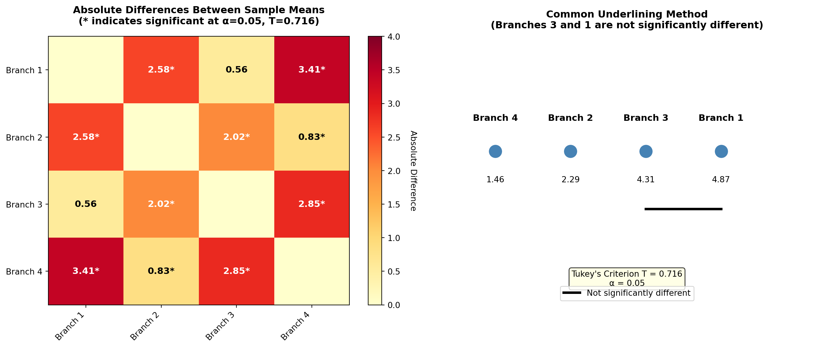
In Example 10.1, Mr. Shade discovered that not all four branches of his bank had the same deposit levels. The logical next step is to determine which ones are different. Because there is an equal number of observations in all four samples (r = 7), either Tukey’s or the LSD method can be used.

11.13.1 Tukey’s Honestly Significant Difference (HSD)

Developed in 1953 by J.W. Tukey, this method requires calculation of Tukey’s criterion, T, as shown in Formula (10.10).

Tukey’s Criterion for Pairwise Comparisons

T = q_{\alpha, c, n-c} \sqrt{\frac{CME}{r}} \quad [10.10]

where: - q has a studentized range distribution with c and n-c degrees of freedom - \alpha is the selected significance level - c is the number of samples or treatments (columns) - n is the total number of observations in all samples combined - r is the number of observations per treatment (equal for balanced designs) - CME is the error mean square from the ANOVA table

11.13.2 Application to First City Bank Example

Recall from Example 10.1: - c = 4 treatments (branches) - n = 28 total observations - r = 7 observations per branch - CME = 0.236 - \alpha = 0.05

Table L (Appendix III) provides critical values for q with \alpha = 0.01 and \alpha = 0.05. If \alpha is set at 0.05, Shade wants the value for q_{0.05, 4, 24}.

In the section of Table L designated for values with \alpha = 0.05: 1. Move across the top row to the first degrees of freedom of 4 2. Move down that column to the second degrees of freedom of 24 3. Find the value: q_{0.05, 4, 24} = 3.90

Then:

T = 3.90 \sqrt{\frac{0.236}{7}} = 3.90 \times 0.1837 = 0.716

11.13.3 Comparing All Pairs of Means

Tukey’s standard criterion of 0.716 is then compared with the absolute difference between each pair of sample means. If any pair of sample means has an absolute difference greater than the T value of 0.716, we can conclude, at a 5% level, that their respective population means are not equal.

The difference between sample means is too large to conclude they come from similar populations. There is only a 5% probability that populations with equal means could produce samples of these sizes with means differing by more than 0.716.

Recall the sample means from Example 10.1: - \bar{X}_1 = 4.87 (Branch 1) - \bar{X}_2 = 2.29 (Branch 2) - \bar{X}_3 = 4.31 (Branch 3) - \bar{X}_4 = 1.46 (Branch 4)

All Pairwise Comparisons:

\begin{aligned} |\bar{X}_1 - \bar{X}_2| &= |4.87 - 2.29| = 2.58 > 0.716^* \\ |\bar{X}_1 - \bar{X}_3| &= |4.87 - 4.31| = 0.56 < 0.716 \\ |\bar{X}_1 - \bar{X}_4| &= |4.87 - 1.46| = 3.41 > 0.716^* \\ |\bar{X}_2 - \bar{X}_3| &= |2.29 - 4.31| = 2.02 > 0.716^* \\ |\bar{X}_2 - \bar{X}_4| &= |2.29 - 1.46| = 0.83 > 0.716^* \\ |\bar{X}_3 - \bar{X}_4| &= |4.31 - 1.46| = 2.85 > 0.716^* \end{aligned}

Asterisks () indicate significant differences at \alpha = 0.05

11.13.4 Interpretation

By comparing the absolute values of each difference between pairs of sample means with T = 0.716, Shade can be 95% confident that only Branches 1 and 3 have equal average deposit levels. All other differences exceed Tukey’s criterion.

11.13.5 Common Underlining Method

These results can be summarized using common underlining, in which lines connecting means show they do not differ significantly. Sample means must first be placed in ordered sequence, generally from lowest to highest:

\begin{array}{cccc} \bar{X}_4 & \bar{X}_2 & \bar{X}_3 & \bar{X}_1 \\ 1.46 & 2.29 & 4.31 & 4.87 \\ & & \underline{\quad\quad\quad} & \end{array}

Because only Branches 1 and 3 do not differ significantly, they are the only ones connected by a common underline.

Figure 11.5: Tukey’s HSD Pairwise Comparisons for Bank Branches

11.14 10.11 Least Significant Difference (LSD) Method

The Least Significant Difference (LSD) method is very similar to Tukey’s method. It compares the LSD criterion with the absolute difference in sample means.

If the design is balanced, the LSD criterion is:

Least Significant Difference for Balanced Designs

LSD = \sqrt{\frac{2(CME) \cdot F_{\alpha, 1, n-c}}{r}} \quad [10.11]

ImportantKey Difference from Tukey

Note that when using the LSD method, F has 1 and n-c degrees of freedom. The first degree of freedom is always 1 for LSD comparisons.

11.14.1 Application to First City Bank Example

In Shade’s case, this is 1 and n - c = 28 - 4 = 24 degrees of freedom. From Table F (Appendix III):

F_{0.05, 1, 24} = 4.26

Then:

LSD = \sqrt{\frac{2(0.236)(4.26)}{7}} = \sqrt{\frac{2.011}{7}} = \sqrt{0.287} = 0.536

11.14.2 Comparing with Tukey’s Method

By comparing the LSD of 0.536 with each of the absolute differences that appeared earlier:

\begin{aligned} |\bar{X}_1 - \bar{X}_2| &= 2.58 > 0.536^* \\ |\bar{X}_1 - \bar{X}_3| &= 0.56 > 0.536^* \\ |\bar{X}_1 - \bar{X}_4| &= 3.41 > 0.536^* \\ |\bar{X}_2 - \bar{X}_3| &= 2.02 > 0.536^* \\ |\bar{X}_2 - \bar{X}_4| &= 0.83 > 0.536^* \\ |\bar{X}_3 - \bar{X}_4| &= 2.85 > 0.536^* \end{aligned}

Shade finds that all values, including the last comparison (Branches 3 and 1), suggest different population means.

TipTukey vs. LSD: Which is More Conservative?

The LSD method is less conservative in that, given any set of conditions, the LSD criterion will be smaller than the Tukey value.

• Tukey’s HSD: More conservative, better control of Type I error across multiple comparisons
• LSD: More liberal, higher power to detect differences but increased Type I error risk

For Mr. Shade’s data: - Tukey’s T = 0.716 (found 5 significant differences) - LSD = 0.536 (found 6 significant differences, including Branch 3 vs. 1)

Recommendation: Use Tukey’s HSD when comparing many treatments to better control family-wise error rate.

11.15 10.12 LSD Method for Unbalanced Designs

If the design is unbalanced (different sample sizes), Tukey’s method and the balanced-design LSD method simply do not apply. Instead, we can use an alternative LSD method.

11.15.1 Alternative LSD for Unbalanced Designs

To compare the j-th and k-th samples, the equation for LSD becomes:

LSD for Unbalanced Designs

LSD_{j,k} = \sqrt{\left[\frac{1}{r_j} + \frac{1}{r_k}\right](CME) \cdot F_{\alpha, c-1, n-c}} \quad [10.12]

where: - r_j is the number of observations in the j-th sample - r_k is the number of observations in the k-th sample

Warning

The LSD value will be different for each pairwise comparison because the number of observations is not the same in each sample.

11.16 Example 10.2: Yosemite National Park Revenue Analysis

More and more Americans seeking to escape urban pressures have caused park admission payments to show a marked increase in weekend camping. Outdoor World recently reported that Yosemite National Park, located in California’s high Sierras, hired an economics consultant to study the park’s financial situation.

Part of the consultant’s effort required a comparison of park revenues from various sources, including camping fees, fishing licenses, and boating permits. Here are data for randomly selected visitors. Determine whether there is a difference in average revenue the park receives from these three activities.

Revenue Data (in dollars)

Visitor	Camping	Fishing	Boating
1	$38.00	$30.00	$19.00
2	32.00	25.00	35.00
3	35.00	31.00	20.00
4	36.00	35.00	22.00
5	38.00	–	25.00
6	32.00	–	–
\bar{X}_j	$35.17	$30.25	$24.20

Note: r_1 = 6, r_2 = 4, r_3 = 5, n = 15 (unbalanced design)

11.16.1 Solution

Assuming \alpha is set at 5%, then F_{\alpha, c-1, n-c} = F_{0.05, 2, 12} = 3.89.

The ANOVA table appears as follows:

ANOVA Summary Table

Source of Variation	Sum of Squares	Degrees of Freedom	Mean Square	F-Value
Between samples (Treatment)	328.0	2	164.0	7.74
Within samples (Error)	254.4	12	21.2
Total Variation	582.4	14

Hypotheses: - H_0: \mu_1 = \mu_2 = \mu_3 - H_A: Not all means are equal

Decision Rule: Do not reject if F \leq 3.89. Reject if F > 3.89.

Conclusion: Reject the null hypothesis since F = 7.74 > 3.89.

11.16.2 Pairwise Comparisons Using Unbalanced LSD

Because we rejected the null hypothesis that average revenues from all three activities are equal, the consultant would want to use pairwise comparisons to determine which differ from the rest.

If \alpha is 5%, F_{0.05, c-1, n-c} = F_{0.05, 2, 12} = 3.89.

Comparison 1: Camping vs. Fishing

\begin{aligned} LSD_{C,F} &= \sqrt{\left[\frac{1}{6} + \frac{1}{4}\right](21.2)(3.89)} \\ &= \sqrt{[0.167 + 0.250](82.47)} \\ &= \sqrt{34.39} \\ &= 5.86 \end{aligned}

Comparison 2: Camping vs. Boating

\begin{aligned} LSD_{C,B} &= \sqrt{\left[\frac{1}{6} + \frac{1}{5}\right](21.2)(3.89)} \\ &= \sqrt{[0.167 + 0.200](82.47)} \\ &= \sqrt{30.27} \\ &= 5.50 \end{aligned}

Comparison 3: Fishing vs. Boating

\begin{aligned} LSD_{F,B} &= \sqrt{\left[\frac{1}{4} + \frac{1}{5}\right](21.2)(3.89)} \\ &= \sqrt{[0.250 + 0.200](82.47)} \\ &= \sqrt{37.11} \\ &= 6.09 \end{aligned}

11.16.3 Evaluating Differences Against LSD Criteria

The differences between means and whether they exceed their respective LSD values are:

\begin{aligned} |\bar{X}_C - \bar{X}_F| &= |35.17 - 30.25| = 4.92 < 5.86 \quad \text{(Not significant)} \\ |\bar{X}_C - \bar{X}_B| &= |35.17 - 24.20| = 10.97 > 5.50^* \quad \text{(Significant)} \\ |\bar{X}_F - \bar{X}_B| &= |30.25 - 24.20| = 6.05 < 6.09 \quad \text{(Not significant)} \end{aligned}

Only Camping and Boating differ significantly.

11.16.4 Common Underlining

Results can be summarized with common underlining after means are placed in ordered array:

\begin{array}{ccc} \bar{X}_B & \bar{X}_F & \bar{X}_C \\ 24.2 & 30.25 & 35.17 \\ \underline{\quad\quad\quad\quad\quad} & \underline{\quad\quad\quad} \end{array}

C:\Users\patod\AppData\Local\Temp\ipykernel_5344\1650205520.py:18: MatplotlibDeprecationWarning: The 'labels' parameter of boxplot() has been renamed 'tick_labels' since Matplotlib 3.9; support for the old name will be dropped in 3.11.
  bp = ax1.boxplot(data_list, labels=activities, patch_artist=True, showmeans=True,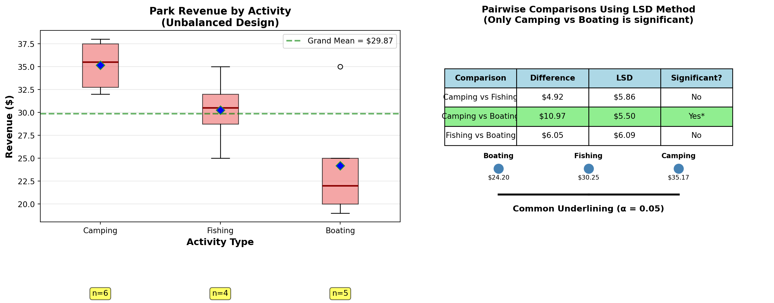

Figure 11.6: Yosemite Park Revenue Comparison with Unbalanced Design

11.16.5 Interpretation

We can conclude at a 5% significance level that only Boating and Camping differ significantly. The park can use this information to make decisions and relieve financial pressure on resources while providing an outdoor experience for modern pioneers.

NoteApparent Contradiction in Underlining

It may seem that the common underlining of the example is self-contradictory. It shows that Boating and Fishing do not differ, and that Fishing and Camping are not different, yet Boating and Camping are different.

The algebraic rule of transitivity says if A = B and B = C, then A = C. However, we are not dealing with equalities here.

We are simply saying: - The difference between Boating and Fishing is not statistically significant - The difference between Fishing and Camping is not statistically significant - But the difference between Boating and Camping is large enough to be statistically significant

This is perfectly valid in statistical hypothesis testing. The strength of evidence differs for different comparisons.

11.17 Section Exercises

Exercise 11.6 (Tukey’s HSD Calculation) A paint manufacturer wants to compare the brightness rating of paint using four different emulsions. Five boards are painted with each emulsion type, and the ratings appear below:

Board	Emulsion 1	Emulsion 2	Emulsion 3	Emulsion 4
1	79	69	83	75
2	82	52	79	78
3	57	62	85	78
4	79	61	78	73
5	83	60	75	71

From ANOVA: F = 8.23 > F_{0.01, 3, 16} = 5.29, so we reject H_0.

1. Is this a balanced or unbalanced design?
2. Calculate Tukey’s criterion T at \alpha = 0.01 (given: CME = 48.5, q_{0.01, 4, 16} = 5.19)
3. Determine which emulsions differ significantly
4. Present results using common underlining
5. Should the manufacturer avoid any particular emulsion?

Exercise 11.7 (Starting Salaries by Field) A study by the American Assembly of Collegiate Schools of Business compared starting salaries (in thousands) of new graduates in various fields:

Graduate	Finance	Marketing	CIS	Quant Methods
1	23.2	22.1	23.3	22.2
2	24.7	19.2	22.1	22.1
3	24.2	21.3	23.4	23.2
4	22.9	19.8	24.2	21.7
5	25.2	17.2	23.1	20.2
6	23.7	18.3	22.7	22.7
7	24.2	17.2	22.8	21.8

At \alpha = 0.05, does there appear to be a difference in average salaries of graduates in different fields?

If ANOVA shows significance: a. Use Tukey’s method to determine which means differ b. Use the LSD method and compare results c. Maintain \alpha = 0.05 and summarize with common underlining

Exercise 11.8 (Plant Production Comparison (Unbalanced)) A medical supply company wants to compare daily average production at three plants. Data collected (in production units):

Toledo: 10, 12, 15, 18, 9, 17, 15, 12, 18
Ottumwa: 15, 17, 18, 12, 13, 11, 12, 11, 12
Crab Apple Cove: 12, 17, 15, 15, 18, 12, 13, 14, 14

1. Is this a balanced or unbalanced design?
2. Conduct ANOVA at \alpha = 0.10
3. If significant, use the appropriate LSD method for pairwise comparisons
4. Which plants have significantly different production levels?

11.18 Section Summary

TipKey Takeaways: Post-Hoc Testing

1. When to use: Only after rejecting H_0 in ANOVA
2. Tukey’s HSD: More conservative, better for many comparisons (balanced designs only)
3. LSD Method: Less conservative, more power (balanced or unbalanced)
4. Common Underlining: Visual method to show which groups are similar
5. Design Balance: Critical factor in choosing the appropriate method
6. Statistical vs. Practical: Significant differences may not always be practically important

11.19 10.13 Two-Way ANOVA: The Randomized Block Design

With one-way analysis of variance, we assumed that only one factor influenced the experimental units—such as deposits at bank branches or revenues at the park. However, we frequently find that a second external influence can impact the experimental units.

For example, interest might be in comparing the average productivity of three types of machines (treatments). However, we observe that when testing these machines, the operator’s skill and experience can affect the machine’s output, creating confusion about which machine is truly better.

Thus, to obtain an uncontaminated and clear picture of machine capability, we must somehow eliminate or correct for the operator’s influence on final output. This simultaneous consideration of two forces requires two-way analysis of variance.

NotePurpose of Two-Way ANOVA

To obtain a decisive measure of treatment capability, we must “block” the extraneous factor by placing observations into homogeneous groups based on the blocking variable (such as years of experience). Observations are thus classified by both blocks and treatments.

11.19.1 The Blocking Concept

Randomized Block Design

An experimental design where observations are grouped into homogeneous blocks to reduce within-treatment variation. The purpose of blocking is to reduce variation within a treatment.

Key Principle: If blocks are performed effectively and based on a factor (such as experience) that truly affects productivity, we obtain a purer measure of the treatment effect.

WarningWhen Blocking Can Be Misleading

If the factor selected for blocking does NOT affect productivity (such as employee social security number, hair color, or gender in contexts where it’s irrelevant), the results can be misleading. It’s important to determine whether blocking is done correctly and whether the blocking factor has actual impact.

11.20 10.14 Business Example: Computer System Selection

A large accounting firm is trying to select an integrated office computer system from among three models currently under study. The final selection will depend on system productivity. Five operators are randomly selected to work with each system.

The Challenge: It’s important to note that the operators’ level of experience in computer handling can affect test results. Therefore, there’s a need to adjust for the impact of experience when determining the relative merits of the computer systems.

The resulting production levels, measured in units per hour, appear in Table 10.3. A higher coded value for experience indicates more years of training.

Table 10.3: Production Levels for Computer Systems

Experience Level	System 1	System 2	System 3	Row Mean \bar{X}_i
1	27	21	25	24.33
2	31	33	35	33.00
3	42	39	39	40.00
4	38	41	37	38.67
5	45	46	45	45.33
Column Mean \bar{X}_j	36.6	36.0	36.2	\bar{X} = 36.27

11.20.1 Understanding the Data Structure

Within a given sample (system), variation in production will occur due to: - Operator experience - Operator competence - Current health status - Other random error factors

In one-way ANOVA, we identified this as error variation. If any of these random factors related to operators materially affect production level, the accounting firm must correct for them.

The firm may believe that an operator’s years of experience significantly affect productivity. However, the firm is interested in system productivity, not employee productivity. Therefore, they must adjust for employee productivity by eliminating the effect of operator variability to obtain a precise, uncontaminated measure of system quality.

11.21 10.15 Partitioning Sums of Squares in Two-Way ANOVA

With two-way ANOVA, the sum of squares total is divided into three parts: 1. Sum of Squares Treatment (SSTR) 2. Sum of Squares Error (SSE) 3. Sum of Squares Blocks (SSBL)

Therefore:

SST = SSTR + SSE + SSBL

SST and SSTR are calculated the same way as in one-way ANOVA. However, SSE is subdivided into a measure for SSE and SSBL.

11.21.1 Sum of Squares for Blocks

Sum of Squares Blocks

SSBL = \sum c_i(\bar{X}_i - \bar{X})^2 \quad [10.13]

where: - c_i is the number of treatments in each block (row) - \bar{X}_i is the mean for each block (row mean) - \bar{X} is the grand mean

The number of treatments in each block, c_i, is multiplied by the squared difference between the mean for each block, \bar{X}_i, and the grand mean. Results are summed for all blocks.

Note

The symbol c_i is used to indicate the number of treatments in a block (row) because treatments are recorded in columns.

11.21.2 Calculation: Computer Systems Example

From Table 10.3:

\begin{aligned} SSBL &= 3(24.33 - 36.27)^2 + 3(33 - 36.27)^2 + 3(40 - 36.27)^2 \\ &\quad + 3(38.67 - 36.27)^2 + 3(45.33 - 36.27)^2 \\ &= 3(142.52) + 3(10.70) + 3(13.91) + 3(5.76) + 3(82.08) \\ &= 427.56 + 32.10 + 41.73 + 17.28 + 246.24 \\ &= 764.91 \end{aligned}

Important

The sum of squares for blocks measures the degree of variation of block means (row means) around the grand mean.

11.21.3 Calculating Other Sums of Squares

Formulas (10.3) and (10.4) give:

\begin{aligned} SST &= \sum \sum (X_{ij} - \bar{X})^2 \\ &= (27 - 36.27)^2 + (31 - 36.27)^2 + \cdots + (45 - 36.27)^2 \\ &= 806.93 \\[10pt] SSTR &= \sum r_j(\bar{X}_j - \bar{X})^2 \\ &= 5(36.6 - 36.27)^2 + 5(36.0 - 36.27)^2 + 5(36.2 - 36.27)^2 \\ &= 5(0.1089) + 5(0.0729) + 5(0.0049) \\ &= 0.93 \end{aligned}

SSE is calculated as:

Sum of Squares Error (Two-Way)

SSE = SST - SSTR - SSBL \quad [10.14]

SSE = 806.93 - 0.93 - 764.91 = 41.09

11.22 10.16 Degrees of Freedom in Two-Way ANOVA

Where there are r blocks and c treatments, there are n = rc observations. The degrees of freedom for each sum of squares from Formula (10.14) are:

\begin{array}{ccccccc} SSE & = & SST & - & SSTR & - & SSBL \\ (r-1)(c-1) & = & (n-1) & - & (c-1) & - & (r-1) \\ (5-1)(3-1) & = & (15-1) & - & (3-1) & - & (5-1) \\ 8 & = & 14 & - & 2 & - & 4 \end{array}

11.23 10.17 Mean Squares and F-Ratios

The total mean square and treatment mean square are, as before, their sum of squares divided by degrees of freedom:

\begin{aligned} CMT &= \frac{SST}{n-1} = \frac{806.93}{14} = 57.64 \\[10pt] CMTR &= \frac{SSTR}{c-1} = \frac{0.93}{2} = 0.47 \end{aligned}

In two-way ANOVA:

Error Mean Square (Two-Way)

CME = \frac{SSE}{(r-1)(c-1)} \quad [10.15]

CME = \frac{41.09}{8} = 5.14

Block Mean Square

CMBL = \frac{SSBL}{r-1} \quad [10.16]

CMBL = \frac{764.91}{4} = 191.23

11.23.1 Two-Way ANOVA Table

Table 10.4: Two-Way ANOVA for Computer Systems

Source of Variation	Sum of Squares	Degrees of Freedom	Mean Square	F-Value
Between samples (Treatment)	0.93	2	0.47	0.09
Between blocks	764.91	4	191.23	37.19
Within samples (Error)	41.09	8	5.14
Total Variation	806.93	14

11.23.2 Calculating F-Values

These calculations are summarized in Table 10.4. F-values are calculated the same way as in one-way ANOVA:

\begin{aligned} F_{\text{treatment}} &= \frac{CMTR}{CME} = \frac{0.47}{5.14} = 0.09 \\[10pt] F_{\text{blocks}} &= \frac{CMBL}{CME} = \frac{191.23}{5.14} = 37.19 \end{aligned}

NoteTwo F-Values Calculated

Note that two F-values are calculated—one using CMTR and one using CMBL. The F-value for CMBL is calculated to determine if blocks were performed effectively.

11.24 10.18 Testing Block Effectiveness

The F-value for CMBL is calculated to determine whether blocks were performed effectively. If blocking is based on a factor that does NOT affect operator productivity, results can be misleading.

Therefore, the accounting firm must test to see if there is a significant difference between block means (row means). If there is no significant difference between average production levels based on blocks (rows), then experience is not a critical factor. In this case, two-way ANOVA should be abandoned, and we would need to return to one-way ANOVA without distinction between experience levels.

11.24.1 Hypothesis Test for Blocks

At a 5% level, the critical F-value for CMBL with 4 and 8 degrees of freedom is obtained from Table G:

F_{0.05, 4, 8} = 3.84

The degrees of freedom 4 and 8 are used because the F-ratio for blocks uses: - CMBL with r - 1 = 4 degrees of freedom (numerator) - CME with (r-1)(c-1) = 8 degrees of freedom (denominator)

Hypotheses: \begin{aligned} H_0 &: \mu_1 = \mu_2 = \mu_3 = \mu_4 = \mu_5 \\ H_A &: \text{Not all block (row) means are equal} \end{aligned}

where \mu_i are the average production levels for each experience level (row).

Decision Rule: “Do not reject if F \leq 3.84. Reject if F > 3.84.”

Conclusion: Because F = 37.19 > 3.84, reject the null hypothesis.

ImportantBlocking is Effective

The accounting firm should conclude that experience levels have an effect on production rates. They must correct for experience using two-way ANOVA.

Figure 11.7: Visualizing the Blocking Effect: Experience Levels vs Production

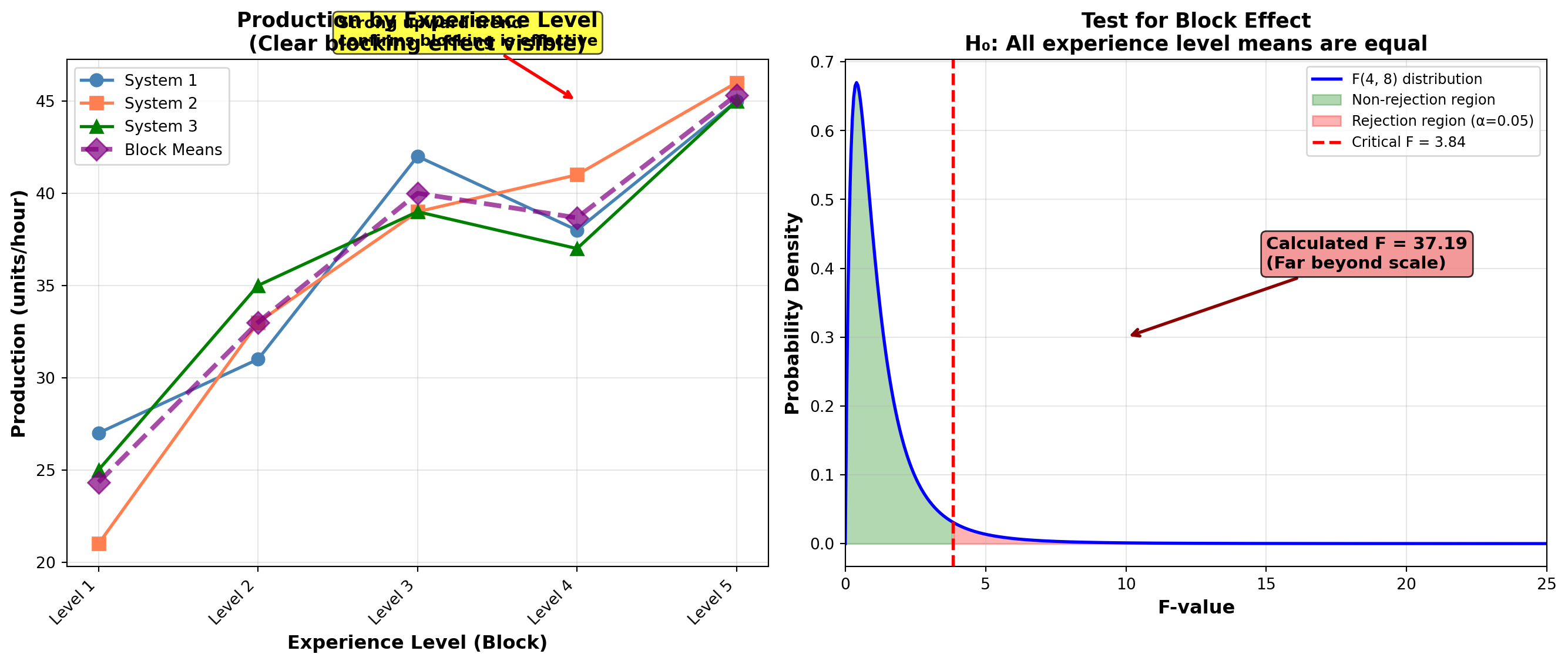
11.25 10.19 Testing Treatment Effects

Now the firm is ready to test the hypothesis they were originally interested in: Is there any difference in average production of computer systems (treatments)?

If the 5% \alpha value is maintained, F_{0.05, 2, 8} = 4.46 is obtained from the table. The degrees of freedom of 2 and 8 are used because the F-ratio for treatments uses: - CMTR with 2 degrees of freedom (numerator) - CME with 8 degrees of freedom (denominator)

Hypotheses: \begin{aligned} H_0 &: \mu_1 = \mu_2 = \mu_3 \\ H_A &: \text{Not all treatment (column) means are equal} \end{aligned}

where \mu_j are the column means for the three computer systems.

Decision Rule: “Do not reject if F \leq 4.46. Reject if F > 4.46.”

Conclusion: Table 10.4 indicates that F = 0.09 < 4.46. Do not reject the null hypothesis.

TipBusiness Interpretation

The firm concludes that average production levels of the three computer systems do not differ, once correction has been made for the experience factor.

Practical Meaning: Employees of different experience levels perform equally well on all machines. It doesn’t matter which computer system they purchase—all three produce similar results when operator experience is accounted for.

11.26 Example 10.3: Manager Performance Evaluation

A recent issue of Fortune magazine described efforts by a major electronics firm to develop a system where employees had the opportunity to evaluate the performance of their supervisors and some management personnel.

Five employees are randomly selected and asked to rate four of their managers on a scale of 10 to 50. The results, along with row and column means, appear in the following table:

Table: Manager Evaluation Ratings

Employee	Manager 1	Manager 2	Manager 3	Manager 4	Row Mean \bar{X}_i
1	31	35	46	38	37.50
2	29	32	45	36	35.50
3	13	17	35	20	21.25
4	28	38	52	39	39.25
5	14	20	40	20	23.50
Column Mean \bar{X}_j	23.0	28.4	43.6	30.6	\bar{X} = 31.4

The electronics firm manager wants to know if there is a difference in average ratings of the four managers.

11.26.1 Solution

The director decides to use two-way ANOVA to test the means. Calculations yield:

\begin{aligned} SST &= \sum \sum (X_{ij} - \bar{X})^2 \\ &= (31 - 31.4)^2 + (29 - 31.4)^2 + \cdots + (20 - 31.4)^2 \\ &= 2,344.8 \\[10pt] SSTR &= \sum r_j(\bar{X}_j - \bar{X})^2 \\ &= 5(23.0 - 31.4)^2 + 5(28.4 - 31.4)^2 + 5(43.6 - 31.4)^2 + 5(30.6 - 31.4)^2 \\ &= 5(70.56) + 5(9.00) + 5(148.84) + 5(0.64) \\ &= 1,145.2 \\[10pt] SSBL &= \sum c_i(\bar{X}_i - \bar{X})^2 \\ &= 4(37.5 - 31.4)^2 + 4(35.5 - 31.4)^2 + 4(21.25 - 31.4)^2 \\ &\quad + 4(39.25 - 31.4)^2 + 4(23.5 - 31.4)^2 \\ &= 4(37.21) + 4(16.81) + 4(103.06) + 4(61.62) + 4(62.41) \\ &= 1,124.4 \\[10pt] SSE &= SST - SSTR - SSBL \\ &= 2,344.8 - 1,145.2 - 1,124.4 \\ &= 75.2 \end{aligned}

Two-Way ANOVA Table:

Source of Variation	Sum of Squares	Degrees of Freedom	Mean Square	F-Value
Between samples (Treatment)	1,145.2	3	381.73	60.91
Between blocks	1,124.4	4	281.10	44.86
Within samples (Error)	75.2	12	6.27
Total Variation	2,344.8	19

11.26.2 Testing Block Effectiveness (Employee Differences)

The director can determine if there is a significant difference in average ratings given by each of the five employees (rows), which will require blocking on employees.

Hypotheses: \begin{aligned} H_0 &: \mu_1 = \mu_2 = \mu_3 = \mu_4 = \mu_5 \\ H_A &: \text{Not all employee (row) means are equal} \end{aligned}

If \alpha = 1\%, the appropriate F-value is F_{0.01, 4, 12} = 5.41.

The F-value related to the test on blocks appears in the ANOVA table as 44.86 > 5.41.

Conclusion: Reject the null hypothesis. The director determines, at a 1% significance level, that average ratings made by the five employees (rows) are different, and blocking is needed.

11.26.3 Testing Treatment Effects (Manager Differences)

The director can now test the initial hypothesis regarding average ratings of the four managers (columns).

Hypotheses: \begin{aligned} H_0 &: \mu_1 = \mu_2 = \mu_3 = \mu_4 \\ H_A &: \text{Not all manager (column) means are equal} \end{aligned}

The F-value of F_{0.01, 3, 12} = 5.95 is less than 60.91.

Conclusion: Reject the null hypothesis at the 1% significance level.

Figure 11.8: Manager Performance Ratings with Employee Blocking

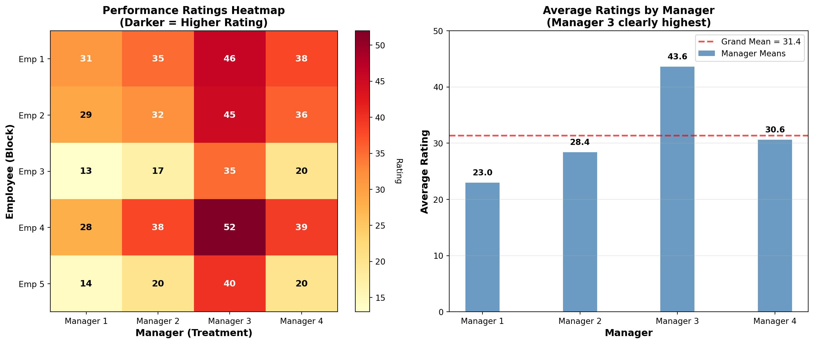
11.26.4 Interpretation

By including a blocking factor, the director was able to detect a significant difference in average manager ratings made by the five employees.

Without the blocking factor: The variation in ratings due to blocks (differences in employee attitudes) would have been included in the error factor SSE. This would have increased SSE and CME.

Impact on F-value: The F-value would have been smaller because F = CMTR/CME. As the F-value decreases, there is a greater probability of not rejecting the null hypothesis.

With two-way ANOVA: The CME is subdivided into variation due to blocks (CMBL) and variation due to error within samples (CME), leading to a more sensitive test.

ImportantKey Insight: Power of Blocking

Two-way ANOVA with blocking: 1. Reduces error variation by accounting for a known source of variability 2. Increases statistical power to detect treatment differences 3. Provides more accurate results when blocking factor truly affects outcomes 4. Requires verification that blocking was effective (test block effect first!)

11.27 Section Exercises

Exercise 11.9 (Pressure Measurement Systems) Three different pressure measurement systems are being compared. Five technicians (with varying experience levels) test each system. Production values (in appropriate units) are:

Technician	System A	System B	System C
1	50	45	45
2	45	30	35
3	30	25	20
4	45	35	40
5	40	30	35

1. Set up the two-way ANOVA table
2. At \alpha = 0.05, test whether blocking on technicians is effective
3. At \alpha = 0.05, test whether systems differ in average performance
4. Interpret results for management decisions

Exercise 11.10 (Accounting Error Analysis) Debits and Credits Inc., an accounting firm in Rocky Top, Tennessee, evaluates new employees by having them complete several accounting statements and compile all errors. You and two other new firm members (Seymore and Gretchen) must fill out six statements. The errors each of you made appear below:

Statement	You	Seymore	Gretchen
1	2	2	3
2	1	3	4
3	0	1	4
4	4	6	5
5	2	3	4
6	1	4	3

At \alpha = 0.05, does one of you appear more or less efficient in accounting skills? If so, which? Block on each statement to account for any difference in difficulty that may exist.

Exercise 11.11 (Production Under Different Payment Methods) Current union-management negotiations focus on the effect payment methods have on worker production. A large firm has five plants. At each, workers are paid by commission, salary, or bonus plan. Three workers randomly selected from all plants each received a different payment method. Their daily production (in units) appears below. Blocking on plants is thought necessary to correct for any production differences.

Plant	Commission	Salary	Bonus
1	25	25	37
2	35	25	50
3	20	22	30
4	30	20	40
5	25	25	35

Based on these data, which payment plan would you suggest to management if the objective is to maximize production? Use \alpha = 0.05.

11.28 Section Summary

TipKey Takeaways: Two-Way ANOVA

1. Purpose: Control for extraneous factor while testing treatment effects
2. Blocking: Groups observations into homogeneous blocks
3. Two Tests: Always test both block effect and treatment effect
4. Order Matters: Test block effectiveness first before interpreting treatment results
5. Increased Power: Proper blocking reduces error variation and increases sensitivity
6. Business Value: Provides clearer, uncontaminated measure of treatment effects

11.29 10.20 Factorial Analysis: Testing for Interaction

In many business and economic applications, researchers need to study the effect of two or more factors simultaneously. For example: - Effect of both advertising budget and price level on sales - Impact of training method and employee experience on productivity - Influence of temperature and humidity on product quality

Factorial analysis allows us to examine these multiple factors together and, most importantly, to detect interaction effects between them.

NoteFactorial Design

A factorial design examines two or more factors simultaneously, with observations at every combination of factor levels. For example, a 3×2 factorial design has: - Factor A with 3 levels - Factor B with 2 levels
- 6 treatment combinations (3 × 2)

11.29.1 What is Interaction?

Interaction

Interaction occurs when the effect of one factor depends on the level of another factor.

Example: Suppose we’re testing the effect of advertising budget (Factor A: Low vs. High) and price level (Factor B: $10 vs. $20) on sales.

• No Interaction: If high advertising always increases sales by $1,000 regardless of price, there is no interaction. The effect of advertising is the same at both price levels.

• Interaction Present: If high advertising increases sales by $2,000 at the $10 price but only by $500 at the $20 price, then interaction exists. The effect of advertising depends on the price level.

11.29.2 Graphical Interpretation of Interaction

No Interaction: Lines are parallel

Sales
  │     High Ad ────────────
  │                ↑
  │               +1000 at both prices
  │                ↓
  │     Low Ad  ─────────────
  │
  └────────────────────────
      $10        $20

Interaction Present: Lines are not parallel (may cross)

Sales
  │     
  │     High Ad @ $10 ──────╲
  │                          ╲
  │                           ╲___ High Ad @ $20
  │     
  │     Low Ad ──────────────────
  │
  └────────────────────────
      $10        $20

11.30 10.21 Example: Computer Systems with Software Packages

An accounting firm wants to evaluate three computer systems (A, B, C) in combination with two software packages (Package 1, Package 2). This creates a 3×2 factorial design with 6 treatment combinations:

• System A with Package 1
• System A with Package 2
• System B with Package 1
• System B with Package 2
• System C with Package 1
• System C with Package 2

Three employees test each combination (3 replicates per cell), producing the following productivity data (units per hour):

Table 10.5: Factorial Design Data

	Package 1			Package 2
System	Rep 1	Rep 2	Rep 3	Rep 1	Rep 2	Rep 3
A	35	37	36	42	45	43
B	40	42	41	38	40	39
C	32	34	33	48	50	49

Cell Means:

System	Package 1	Package 2	Row Mean
A	36.0	43.3	39.7
B	41.0	39.0	40.0
C	33.0	49.0	41.0
Column Mean	36.7	43.8	\bar{X} = 40.2

11.30.1 Three Hypotheses in Factorial ANOVA

With factorial designs, we test three hypotheses:

1. Main Effect of Factor A (Systems) \begin{aligned} H_0 &: \mu_A = \mu_B = \mu_C \\ H_A &: \text{Not all system means are equal} \end{aligned}

2. Main Effect of Factor B (Software) \begin{aligned} H_0 &: \mu_1 = \mu_2 \\ H_A &: \text{Package means are not equal} \end{aligned}

3. Interaction Effect (System × Software) \begin{aligned} H_0 &: \text{No interaction between systems and software} \\ H_A &: \text{Interaction exists} \end{aligned}

11.30.2 Calculating Sums of Squares for Factorial Design

For a factorial design with factor A at a levels, factor B at b levels, and r replicates per cell:

Total Sum of Squares: SST = \sum\sum\sum (X_{ijk} - \bar{X})^2

Sum of Squares for Factor A: SS_A = br \sum (\bar{X}_{i\cdot\cdot} - \bar{X})^2

where \bar{X}_{i\cdot\cdot} is the mean for level i of factor A, and b is the number of levels of factor B.

Sum of Squares for Factor B: SS_B = ar \sum (\bar{X}_{\cdot j\cdot} - \bar{X})^2

where \bar{X}_{\cdot j\cdot} is the mean for level j of factor B, and a is the number of levels of factor A.

Sum of Squares for Interaction: SS_{AB} = r \sum\sum (\bar{X}_{ij\cdot} - \bar{X}_{i\cdot\cdot} - \bar{X}_{\cdot j\cdot} + \bar{X})^2

Sum of Squares Error: SSE = SST - SS_A - SS_B - SS_{AB}

11.30.3 Calculations for Computer Systems Example

With a = 3 systems, b = 2 packages, r = 3 replicates, n = 18 total observations:

\begin{aligned} SST &= (35-40.2)^2 + (37-40.2)^2 + \cdots + (49-40.2)^2 \\ &= 666.0 \\[10pt] SS_A &= (2)(3)[(39.7-40.2)^2 + (40.0-40.2)^2 + (41.0-40.2)^2] \\ &= 6[0.25 + 0.04 + 0.64] \\ &= 5.6 \\[10pt] SS_B &= (3)(3)[(36.7-40.2)^2 + (43.8-40.2)^2] \\ &= 9[12.25 + 12.96] \\ &= 226.9 \\[10pt] SS_{AB} &= 3[(36.0-39.7-36.7+40.2)^2 + (43.3-39.7-43.8+40.2)^2 \\ &\quad + (41.0-40.0-36.7+40.2)^2 + (39.0-40.0-43.8+40.2)^2 \\ &\quad + (33.0-41.0-36.7+40.2)^2 + (49.0-41.0-43.8+40.2)^2] \\ &= 3[0.64 + 0 + 20.25 + 30.25 + 22.09 + 20.25] \\ &= 3[93.48] \\ &= 280.4 \\[10pt] SSE &= 666.0 - 5.6 - 226.9 - 280.4 \\ &= 153.1 \end{aligned}

11.30.4 Degrees of Freedom

• Factor A: df_A = a - 1 = 3 - 1 = 2
• Factor B: df_B = b - 1 = 2 - 1 = 1
• Interaction: df_{AB} = (a-1)(b-1) = (2)(1) = 2
• Error: df_E = ab(r-1) = (3)(2)(3-1) = 12
• Total: df_T = n - 1 = 18 - 1 = 17

11.30.5 Mean Squares and F-Ratios

\begin{aligned} MS_A &= \frac{SS_A}{df_A} = \frac{5.6}{2} = 2.8 \\[10pt] MS_B &= \frac{SS_B}{df_B} = \frac{226.9}{1} = 226.9 \\[10pt] MS_{AB} &= \frac{SS_{AB}}{df_{AB}} = \frac{280.4}{2} = 140.2 \\[10pt] MSE &= \frac{SSE}{df_E} = \frac{153.1}{12} = 12.76 \\[10pt] F_A &= \frac{MS_A}{MSE} = \frac{2.8}{12.76} = 0.22 \\[10pt] F_B &= \frac{MS_B}{MSE} = \frac{226.9}{12.76} = 17.78 \\[10pt] F_{AB} &= \frac{MS_{AB}}{MSE} = \frac{140.2}{12.76} = 10.99 \end{aligned}

Table 10.6: Two-Way Factorial ANOVA

Source	SS	df	MS	F-Value
Factor A (Systems)	5.6	2	2.8	0.22
Factor B (Software)	226.9	1	226.9	17.78
Interaction (A×B)	280.4	2	140.2	10.99
Error	153.1	12	12.76
Total	666.0	17

11.30.6 Hypothesis Testing at α = 0.05

Test 1: Interaction Effect (Test this first!) - H_0: No interaction between systems and software - F_{0.05, 2, 12} = 3.89 - Decision: F_{AB} = 10.99 > 3.89 → Reject H_0 - Conclusion: Significant interaction exists

Test 2: Main Effect of Software (Factor B) - H_0: \mu_1 = \mu_2 (Package means equal) - F_{0.05, 1, 12} = 4.75 - Decision: F_B = 17.78 > 4.75 → Reject H_0 - Conclusion: Package means differ significantly

Test 3: Main Effect of Systems (Factor A) - H_0: \mu_A = \mu_B = \mu_C (System means equal) - F_{0.05, 2, 12} = 3.89 - Decision: F_A = 0.22 < 3.89 → Do not reject H_0 - Conclusion: No significant difference in system means

WarningInterpreting Results with Interaction

When significant interaction exists, we must be careful about interpreting main effects. The interaction tells us that the effect of one factor depends on the level of the other factor.

In this case: - Package 2 works much better with System C (mean = 49.0) - Package 1 works better with System B (mean = 41.0) - The “best” software package depends on which system you’re using!

Figure 11.9: Interaction Plot: Computer Systems and Software Packages

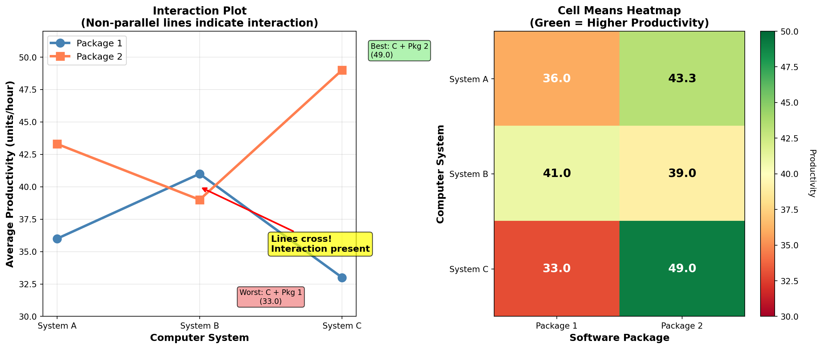
11.30.7 Business Interpretation

The significant interaction reveals important insights:

1. System C with Package 2: Highest productivity (49.0 units/hour)
2. System C with Package 1: Lowest productivity (33.0 units/hour)
3. System B with Package 1: Good performance (41.0 units/hour)
4. System B with Package 2: Moderate performance (39.0 units/hour)

Recommendation: The firm should NOT make a blanket decision about “which system is best” or “which software is best.” Instead, they should recognize that: - If using Package 2, choose System C - If using Package 1, choose System B - System A performs moderately with both packages

11.31 10.22 Latin Square Design

There are occasions when it’s necessary to block on two extraneous variables simultaneously. The Latin Square design accomplishes this while maintaining efficiency.

NoteLatin Square Design

A Latin Square design blocks on two factors simultaneously, with: - r treatments under study - r levels of blocking factor 1 (rows) - r levels of blocking factor 2 (columns) - Each treatment appears exactly once in each row and once in each column - Total observations: r^2

The design is called a “square” because it requires an equal number of treatments, row blocks, and column blocks (r \times r = r^2 observations). It’s called “Latin” because letters like A, B, C are traditionally used to denote treatments.

11.31.1 Example: Computer Systems with Two Blocking Factors

Returning to the computer systems example, suppose the firm wants to test three systems (A, B, C) but needs to control for: - Employee experience level (3 levels) - Time of day (Morning, Afternoon, Evening)

This creates a 3×3 Latin Square:

Table 10.7: Latin Square Design for Computer Systems

	Time of Day
Experience	Morning	Afternoon	Evening	Row Total
1	B/15	A/18	C/11	44
2	C/12	B/20	A/9	41
3	A/17	C/19	B/10	46
Column Total	44	57	30	131

Treatment Totals: - \sum A = 18 + 9 + 17 = 44 - \sum B = 15 + 20 + 10 = 45 - \sum C = 11 + 12 + 19 = 42

11.31.2 Formulas for Latin Square Analysis

Sum of Squares for Row Blocks (SSBR): SSBR = \frac{\sum(\text{row sum})^2}{r} - \frac{(\sum X_i)^2}{r^2} \quad [10.17]

Sum of Squares for Column Blocks (SSBC): SSBC = \frac{\sum(\text{column sum})^2}{r} - \frac{(\sum X_i)^2}{r^2} \quad [10.18]

Sum of Squares for Treatments (SSTR): SSTR = \frac{\sum(\text{treatment sum})^2}{r} - \frac{(\sum X_i)^2}{r^2} \quad [10.19]

Total Sum of Squares: SST = \sum(X_i)^2 - \frac{(\sum X_i)^2}{r^2} \quad [10.20]

Sum of Squares Error: SSE = SST - SSTR - SSBC - SSBR \quad [10.21]

11.31.3 Calculations for Computer Systems Example

With r = 3 treatments:

\begin{aligned} SSBR &= \frac{(44)^2 + (41)^2 + (46)^2}{3} - \frac{(131)^2}{9} \\ &= \frac{1,936 + 1,681 + 2,116}{3} - \frac{17,161}{9} \\ &= \frac{5,733}{3} - 1,906.78 \\ &= 4.222 \\[10pt] SSBC &= \frac{(44)^2 + (57)^2 + (30)^2}{3} - \frac{(131)^2}{9} \\ &= \frac{1,936 + 3,249 + 900}{3} - 1,906.78 \\ &= 2,028.33 - 1,906.78 \\ &= 121.556 \\[10pt] SSTR &= \frac{(44)^2 + (45)^2 + (42)^2}{3} - \frac{(131)^2}{9} \\ &= \frac{1,936 + 2,025 + 1,764}{3} - 1,906.78 \\ &= 1,908.33 - 1,906.78 \\ &= 1.556 \\[10pt] SST &= (15)^2 + (12)^2 + (17)^2 + \cdots + (10)^2 - \frac{(131)^2}{9} \\ &= 2,045 - 1,906.78 \\ &= 138.222 \\[10pt] SSE &= 138.222 - 1.556 - 121.556 - 4.222 \\ &= 10.888 \end{aligned}

11.31.4 Degrees of Freedom for Latin Square

• Row blocks: df_{BR} = r - 1 = 3 - 1 = 2
• Column blocks: df_{BC} = r - 1 = 3 - 1 = 2
• Treatments: df_{TR} = r - 1 = 3 - 1 = 2
• Error: df_E = (r-1)(r-2) = (3-1)(3-2) = 2
• Total: df_T = r^2 - 1 = 9 - 1 = 8

11.31.5 Latin Square ANOVA Table

Table 10.8: Latin Square ANOVA for Computer Systems

Source of Variation	SS	df	MS	F-Value
Row blocks (Experience)	4.222	2	2.111	0.39
Column blocks (Time)	121.556	2	60.778	11.16
Treatments (Systems)	1.556	2	0.778	0.14
Error	10.888	2	5.444
Total	138.222	8

11.31.6 Hypothesis Testing for Latin Square

At \alpha = 0.05, the critical F-value with 2 and 2 degrees of freedom is F_{0.05, 2, 2} = 19.00.

Test 1: Row Blocks (Experience) - H_0: No difference in mean productivity across experience levels - F = 0.39 < 19.00 → Do not reject H_0 - Conclusion: Row blocking not effective

Test 2: Column Blocks (Time of Day) - H_0: No difference in mean productivity across time periods - F = 11.16 < 19.00 → Do not reject H_0 - Conclusion: Column blocking not effective (though F is larger)

Test 3: Treatments (Computer Systems) - H_0: \mu_A = \mu_B = \mu_C - F = 0.14 < 19.00 → Do not reject H_0 - Conclusion: No significant difference in system productivity

TipBusiness Interpretation

After adjusting for employee experience and time of day, the three computer systems show no significant difference in average productivity. The firm can select any system based on other criteria such as cost, reliability, or vendor support.

Note: The small sample size (only 9 observations) makes it difficult to detect differences. With df_E = 2, the critical F-value is very high (19.00), requiring large differences to be statistically significant.

Figure 11.10: Latin Square Design Visualization

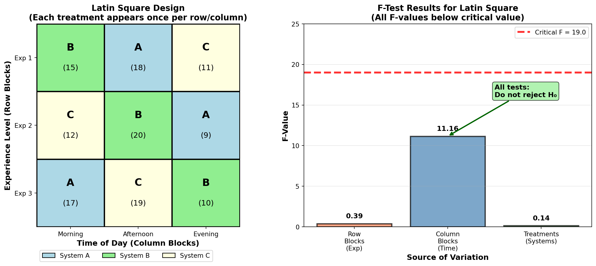
11.32 Section Exercises

Exercise 11.12 (Wire Manufacturing: Chemical Mixtures) A wire manufacturer wants to compare tensile strength using three different chemical mixtures (A, B, C). It’s necessary to control for the type of furnace used to “melt” the mixture and the temperature at which it was melted. Using the following data in a Latin Square design, what conclusion do you draw for the manufacturer? Use \alpha = 1\%.

	Temperature
Furnace	Low	Medium	High
1	A/40	B/42	C/18
2	B/70	C/19	A/45
3	C/20	A/51	B/27

Exercise 11.13 (Electric Fork Sales by Brand and Location) As marketing director, you’re interested in comparing revenues from three brands—“Good,” “Better,” “Best”—of electric forks your company sells. You want to control for the region of the country where the store is located and the type of store where the sale was made. Your assistant collected data for monthly sales (in hundreds of dollars) as shown below. Perform the test yourself and report findings to your assistant. Use \alpha = 1\%.

	Region
Store	Northeast	Southeast	Central
Discount	Good/4.2	Better/9.0	Best/12.9
Hardware	Better/7.3	Best/11.1	Good/11.3
Mall	Best/8.0	Good/9.4	Better/10.7

Exercise 11.14 (Faculty Salaries by Department) A researcher collects data on faculty salaries to determine whether there’s a difference in average income for those in business, social sciences, and natural sciences. They must eliminate extraneous effects of rank and school size. Using the information below regarding salaries (in thousands of dollars), what do you suppose the results are? Use \alpha = 1\% and interpret.

	School Size
Rank	Small	Medium	Large
Assistant Prof	Bus/65	SS/60	NS/78
Associate Prof	SS/72	NS/81	Bus/79
Full Professor	NS/82	Bus/73	SS/79

Where: Bus = Business, SS = Social Sciences, NS = Natural Sciences

11.33 Solved Problems

11.33.1 Problem 1: Regional Gasoline Tax Analysis

Context: A consumer study published results of a survey on driving habits in the United States. The data contained gasoline taxes per household for all 50 states. Six states were randomly chosen from four regions to determine if there’s any difference in average annual gasoline tax across regions.

Data: Annual Gasoline Tax by Region (in dollars)

State	North (1)	South (2)	West (3)	Midwest (4)
1	$293	$121	$114	$136
2	280	116	176	164
3	283	223	224	117
4	242	238	183	153
5	268	118	159	152
6	184	222	149	108
Mean	258.3	173.0	167.5	138.3

Grand Mean: \bar{X} = 184.3

Objective: Test at the 5% level whether residents of the four regions pay the same average amount in federal gasoline taxes.

11.33.1.1 Solution

Hypotheses: \begin{aligned} H_0 &: \mu_1 = \mu_2 = \mu_3 = \mu_4 \\ H_A &: \text{Not all regional means are equal} \end{aligned}

Calculations:

\begin{aligned} SST &= \sum\sum (X_{ij} - \bar{X})^2 \\ &= (293 - 184.3)^2 + (280 - 184.3)^2 + \cdots + (108 - 184.3)^2 \\ &= 83,515 \\[10pt] SSTR &= \sum r_j(\bar{X}_j - \bar{X})^2 \\ &= 6(258.3 - 184.3)^2 + 6(173.0 - 184.3)^2 \\ &\quad + 6(167.5 - 184.3)^2 + 6(138.3 - 184.3)^2 \\ &= 6(5,476.36) + 6(127.69) + 6(282.24) + 6(2,116.36) \\ &= 48,023 \\[10pt] SSE &= SST - SSTR \\ &= 83,515 - 48,023 \\ &= 35,492 \\[10pt] CMTR &= \frac{SSTR}{c-1} = \frac{48,023}{3} = 16,008 \\[10pt] CME &= \frac{SSE}{n-c} = \frac{35,492}{24-4} = \frac{35,492}{20} = 1,775 \end{aligned}

F-Ratio: F = \frac{CMTR}{CME} = \frac{16,008}{1,775} = 9.02

Decision Rule: At \alpha = 0.05 with df = (3, 20): F_{0.05, 3, 20} = 3.10

Conclusion: Since F = 9.02 > 3.10, reject H_0 at the 5% significance level.

Interpretation: We conclude that the average gasoline tax is NOT the same across the four regions. There are significant differences in the tax burden faced by residents in different parts of the country.

11.33.2 Problem 2: Pairwise Comparisons - Which Regions Differ?

Objective: Using both Tukey’s method and LSD, determine which specific regions have different average taxes.

11.33.2.1 Solution

Step 1: Calculate absolute differences between sample means

\begin{aligned} |\bar{X}_1 - \bar{X}_2| &= |258.3 - 173.0| = 85.3 \\ |\bar{X}_1 - \bar{X}_3| &= |258.3 - 167.5| = 90.8 \\ |\bar{X}_1 - \bar{X}_4| &= |258.3 - 138.3| = 120.0 \\ |\bar{X}_2 - \bar{X}_3| &= |173.0 - 167.5| = 5.5 \\ |\bar{X}_2 - \bar{X}_4| &= |173.0 - 138.3| = 34.7 \\ |\bar{X}_3 - \bar{X}_4| &= |167.5 - 138.3| = 29.2 \end{aligned}

Step 2: Tukey’s HSD Method

T = q_{\alpha, c, n-c} \sqrt{\frac{CME}{r}}

At \alpha = 0.05: q_{0.05, 4, 20} = 3.96

T = 3.96 \sqrt{\frac{1,775}{6}} = 3.96(17.20) = 68.11

Interpretation: Any difference greater than 68.11 is significant.

Comparing to calculated differences: - |\bar{X}_1 - \bar{X}_2| = 85.3 > 68.11 ✓ Significant - |\bar{X}_1 - \bar{X}_3| = 90.8 > 68.11 ✓ Significant - |\bar{X}_1 - \bar{X}_4| = 120.0 > 68.11 ✓ Significant - |\bar{X}_2 - \bar{X}_3| = 5.5 < 68.11 — Not significant - |\bar{X}_2 - \bar{X}_4| = 34.7 < 68.11 — Not significant - |\bar{X}_3 - \bar{X}_4| = 29.2 < 68.11 — Not significant

Conclusion: The North region (Region 1) has significantly higher average taxes than all other three regions. Regions 2, 3, and 4 do not differ significantly from each other.

Step 3: LSD Method

LSD = \sqrt{\frac{2(CME) \cdot F_{\alpha, 1, n-c}}{r}}

F_{0.05, 1, 20} = 4.35

LSD = \sqrt{\frac{2(1,775)(4.35)}{6}} = \sqrt{2,573.75} = 50.73

Interpretation: Any difference greater than 50.73 is significant.

Comparing to calculated differences: - |\bar{X}_1 - \bar{X}_2| = 85.3 > 50.73 ✓ Significant - |\bar{X}_1 - \bar{X}_3| = 90.8 > 50.73 ✓ Significant - |\bar{X}_1 - \bar{X}_4| = 120.0 > 50.73 ✓ Significant - |\bar{X}_2 - \bar{X}_3| = 5.5 < 50.73 — Not significant - |\bar{X}_2 - \bar{X}_4| = 34.7 < 50.73 — Not significant - |\bar{X}_3 - \bar{X}_4| = 29.2 < 50.73 — Not significant

Common Underlining:

  Region 4   Region 3   Region 2   Region 1
  138.3      167.5      173.0      258.3
  ________________________________

Policy Implication: Motorists in the North bear the heaviest tax burden. The other three regions have statistically similar tax levels and could potentially be grouped together for policy purposes.

11.33.3 Problem 3: Production Levels with Blocking on Weeks

Context: As production supervisor at Acme Ltd., Melvin Moore wants to compare production levels at four plants. Weekly data on production levels (in tons) were collected over seven weeks (four weeks in August and three weeks in September).

Data: Weekly Production by Plant

Week	Plant 1	Plant 2	Plant 3	Plant 4	Row Mean
1	42.7	38.3	42.9	30.1	38.5
2	47.3	35.1	38.2	37.5	39.5
3	57.3	42.7	49.9	47.8	49.4
4	63.1	58.2	59.3	53.9	58.6
5	49.2	32.7	45.7	33.8	40.4
6	51.2	30.1	48.3	38.7	42.1
7	48.0	31.1	45.2	39.7	41.0
Col Mean	51.3	38.3	47.1	40.2	\bar{X} = 44.23

Note: Melvin initially performed one-way ANOVA and found significant differences. However, he realized the same seven weeks were used for all plants, suggesting blocking on weeks might be appropriate.

11.33.3.1 Solution

Calculations for Two-Way ANOVA:

From one-way analysis: SST = 2,276.1 and SSTR = 761.4

\begin{aligned} SSBL &= \sum c_i(\bar{X}_i - \bar{X})^2 \\ &= 4(38.5 - 44.23)^2 + 4(39.5 - 44.23)^2 + 4(49.4 - 44.23)^2 \\ &\quad + 4(58.6 - 44.23)^2 + 4(40.4 - 44.23)^2 \\ &\quad + 4(42.1 - 44.23)^2 + 4(41.0 - 44.23)^2 \\ &= 4(32.86 + 22.37 + 26.73 + 206.56 + 14.67 + 4.54 + 10.43) \\ &= 4(319.16) \\ &= 1,276.6 \\[10pt] SSE &= SST - SSTR - SSBL \\ &= 2,276.1 - 761.4 - 1,276.6 \\ &= 238.1 \\[10pt] CMTR &= \frac{SSTR}{c-1} = \frac{761.4}{3} = 253.8 \\[10pt] CMBL &= \frac{SSBL}{r-1} = \frac{1,276.6}{6} = 212.8 \\[10pt] CME &= \frac{SSE}{(r-1)(c-1)} = \frac{238.1}{(6)(3)} = \frac{238.1}{18} = 13.2 \end{aligned}

Two-Way ANOVA Table:

Source	SS	df	MS	F-Value
Between samples (Treatment)	761.4	3	253.8	19.23
Between blocks (Weeks)	1,276.6	6	212.8	16.12
Within samples (Error)	238.1	18	13.2
Total	2,276.1	27

Test 1: Block Effectiveness (α = 0.05) - H_0: No difference in average production across weeks - F_{0.05, 6, 18} = 2.66 - Decision: F = 16.12 > 2.66 → Reject H_0 - Conclusion: Average production varies significantly across weeks. Blocking is necessary.

Test 2: Treatment Effects (α = 0.05) - H_0: \mu_1 = \mu_2 = \mu_3 = \mu_4 (Plant means equal) - F_{0.05, 3, 18} = 3.16 - Decision: F = 19.23 > 3.16 → Reject H_0 - Conclusion: Significant differences exist in average production levels across plants.

Interpretation: By blocking on weeks, Melvin accounts for variation due to different time periods (perhaps seasonal effects, holidays, etc.). Even after accounting for this variation, significant differences among plant production levels remain. Melvin can now use LSD or Tukey’s method to determine which specific plants differ.

11.33.4 Problem 4: Circle Trucking - Latin Square Design

Context: Circle Trucking Company wants to determine if average driving time is the same for three routes. The traffic director needs to control for both weather conditions and driver skill. Three weather levels (Poor, Fair, Good) and three drivers with varying abilities are identified. Each driver covers each route under each weather condition.

Data: Driving Times (minutes) - Latin Square

	Weather
Driver	Poor	Fair	Good	Row Total
1	A/20	C/18	B/17	55
2	C/22	B/10	A/10	42
3	B/18	A/9	C/8	35
Col Total	60	37	35	132

Treatment Totals: - \sum A = 20 + 10 + 9 = 39 - \sum B = 17 + 10 + 18 = 45 - \sum C = 18 + 22 + 8 = 48

11.33.4.1 Solution

Using Latin Square formulas with r = 3:

\begin{aligned} SSBR &= \frac{(55)^2 + (42)^2 + (35)^2}{3} - \frac{(132)^2}{9} \\ &= \frac{3,025 + 1,764 + 1,225}{3} - \frac{17,424}{9} \\ &= \frac{6,014}{3} - 1,936 \\ &= 2,004.67 - 1,936 \\ &= 68.667 \\[10pt] SSBC &= \frac{(60)^2 + (37)^2 + (35)^2}{3} - \frac{(132)^2}{9} \\ &= \frac{3,600 + 1,369 + 1,225}{3} - 1,936 \\ &= \frac{6,194}{3} - 1,936 \\ &= 2,064.67 - 1,936 \\ &= 128.667 \\[10pt] SSTR &= \frac{(39)^2 + (45)^2 + (48)^2}{3} - \frac{(132)^2}{9} \\ &= \frac{1,521 + 2,025 + 2,304}{3} - 1,936 \\ &= \frac{5,850}{3} - 1,936 \\ &= 1,950 - 1,936 \\ &= 14.000 \\[10pt] SST &= (20)^2 + (22)^2 + (18)^2 + \cdots + (8)^2 - \frac{(132)^2}{9} \\ &= 2,166 - 1,936 \\ &= 230.000 \\[10pt] SSE &= SST - SSTR - SSBC - SSBR \\ &= 230 - 14 - 128.667 - 68.667 \\ &= 18.666 \end{aligned}

Latin Square ANOVA Table:

Source	SS	df	MS	F-Value
Row blocks (Drivers)	68.667	2	34.333	3.68
Column blocks (Weather)	128.667	2	64.333	6.89
Treatments (Routes)	14.000	2	7.000	0.75
Error	18.666	2	9.333
Total	230.000	8

Hypothesis Tests (α = 0.05)

Critical F-value: F_{0.05, 2, 2} = 19.00

Test 1: Driver Effect - F = 3.68 < 19.00 → Do not reject H_0

Test 2: Weather Effect - F = 6.89 < 19.00 → Do not reject H_0

Test 3: Route Effect - F = 0.75 < 19.00 → Do not reject H_0

Conclusion: At the 5% significance level, there is no significant difference in average driving time across the three routes, after controlling for driver skill and weather conditions. Circle Trucking can use any of the three routes with confidence that average driving times are statistically equivalent.

Note: The high critical F-value (19.00) with only 2 error degrees of freedom makes it difficult to detect differences. A larger study would be recommended for more conclusive results.

11.34 Formula Summary

11.34.1 One-Way ANOVA

Grand Mean: \bar{X} = \frac{\sum X_{ij}}{n}

Sums of Squares: \begin{aligned} SST &= \sum\sum (X_{ij} - \bar{X})^2 \\ SSTR &= \sum r_j(\bar{X}_j - \bar{X})^2 \\ SSE &= SST - SSTR \end{aligned}

Mean Squares: \begin{aligned} CMTR &= \frac{SSTR}{c-1} \\ CME &= \frac{SSE}{n-c} \end{aligned}

F-Ratio: F = \frac{CMTR}{CME}

Tukey’s HSD: T = q_{\alpha, c, n-c} \sqrt{\frac{CME}{r}}

LSD (Balanced): LSD = \sqrt{\frac{2 \cdot CME \cdot F_{\alpha, 1, n-c}}{r}}

LSD (Unbalanced): LSD_{j,k} = \sqrt{\left(\frac{1}{r_j} + \frac{1}{r_k}\right) \cdot CME \cdot F_{\alpha, c-1, n-c}}

11.34.2 Two-Way ANOVA (Randomized Block Design)

Sum of Squares for Blocks: SSBL = \sum c_i(\bar{X}_i - \bar{X})^2

Partitioning: SST = SSTR + SSBL + SSE

Mean Squares: \begin{aligned} CMTR &= \frac{SSTR}{c-1} \\ CMBL &= \frac{SSBL}{r-1} \\ CME &= \frac{SSE}{(r-1)(c-1)} \end{aligned}

F-Ratios: \begin{aligned} F_{\text{treatment}} &= \frac{CMTR}{CME} \\ F_{\text{blocks}} &= \frac{CMBL}{CME} \end{aligned}

11.34.3 Factorial Analysis

Sum of Squares for Factor A: SS_A = br \sum (\bar{X}_{i\cdot\cdot} - \bar{X})^2

Sum of Squares for Factor B: SS_B = ar \sum (\bar{X}_{\cdot j\cdot} - \bar{X})^2

Sum of Squares for Interaction: SS_{AB} = r \sum\sum (\bar{X}_{ij\cdot} - \bar{X}_{i\cdot\cdot} - \bar{X}_{\cdot j\cdot} + \bar{X})^2

Partitioning: SST = SS_A + SS_B + SS_{AB} + SSE

Degrees of Freedom: \begin{aligned} df_A &= a - 1 \\ df_B &= b - 1 \\ df_{AB} &= (a-1)(b-1) \\ df_E &= ab(r-1) \end{aligned}

11.34.4 Latin Square Design

Row Blocks: SSBR = \frac{\sum(\text{row sum})^2}{r} - \frac{(\sum X_i)^2}{r^2}

Column Blocks: SSBC = \frac{\sum(\text{column sum})^2}{r} - \frac{(\sum X_i)^2}{r^2}

Treatments: SSTR = \frac{\sum(\text{treatment sum})^2}{r} - \frac{(\sum X_i)^2}{r^2}

Total: SST = \sum(X_i)^2 - \frac{(\sum X_i)^2}{r^2}

Error: SSE = SST - SSTR - SSBC - SSBR

Degrees of Freedom: \begin{aligned} df_{BR} &= r - 1 \\ df_{BC} &= r - 1 \\ df_{TR} &= r - 1 \\ df_E &= (r-1)(r-2) \end{aligned}

11.35 Chapter Summary

11.35.1 Key Concepts Mastered

1. One-Way ANOVA: Tests whether means from three or more populations are equal by partitioning total variation into treatment variation and error variation.

2. F-Distribution: The ratio of two variance estimates (CMTR/CME) follows an F-distribution under the null hypothesis. Large F-values provide evidence against equal means.

3. Pairwise Comparisons: After rejecting the ANOVA null hypothesis, Tukey’s HSD or LSD methods identify which specific means differ.

4. Two-Way ANOVA: Controls for one extraneous variable (blocking factor) while testing treatment effects, increasing statistical power when blocking is effective.

5. Factorial Analysis: Examines two or more factors simultaneously and detects interaction effects, revealing whether the effect of one factor depends on levels of another.

6. Latin Square: Controls for two extraneous variables simultaneously with an efficient design requiring r^2 observations for r treatments.

11.35.2 Decision Flowchart

graph TD
    A[Start: Comparing Means] --> B{How many<br/>treatments?}
    B -->|Two| C[Use t-test<br/>Chapter 9]
    B -->|Three or more| D{Any known<br/>extraneous<br/>factors?}
    
    D -->|None| E[One-Way ANOVA]
    D -->|One factor| F[Two-Way ANOVA<br/>Randomized Block]
    D -->|Two factors| G{Same factor<br/>as treatment?}
    
    G -->|No| H[Latin Square]
    G -->|Yes| I{Interested in<br/>interaction?}
    
    I -->|Yes| J[Factorial ANOVA]
    I -->|No| K[Two-Way ANOVA<br/>with both factors]
    
    E --> L[Test F-ratio]
    F --> M[Test blocks first]
    H --> N[Test all three<br/>sources]
    J --> O[Test interaction<br/>first]
    
    L --> P{Reject H0?}
    M --> Q{Blocks<br/>effective?}
    
    P -->|Yes| R[Pairwise<br/>Comparisons]
    P -->|No| S[Conclude means<br/>are equal]
    
    Q -->|Yes| T[Test treatments]
    Q -->|No| U[Use one-way<br/>instead]
    
    R --> V[Tukey's or LSD]
    T --> P

ANOVA Method Selection Decision Flowchart

11.35.3 When to Use Each Method

Method	Use When	Example
One-Way ANOVA	Comparing ≥3 treatments, no known confounding variables	Compare sales across 4 regions
Two-Way ANOVA	Comparing treatments while controlling for 1 extraneous factor	Compare productivity of 3 machines, blocking on operator experience
Factorial ANOVA	Testing 2+ factors simultaneously, interested in interaction	Compare effectiveness of advertising budget × price level on sales
Latin Square	Comparing treatments while controlling for 2 extraneous factors	Compare 3 routes while controlling for driver skill and weather

11.35.4 Critical Assumptions

All ANOVA methods assume: 1. Normality: Populations are approximately normally distributed 2. Equal Variances: Population variances are equal (homoscedasticity) 3. Independence: Observations are independent

Violations of these assumptions may invalidate results. Use appropriate diagnostics and transformations when necessary.

11.35.5 Resolving the Opening Scenario

Returning to our opening scenario about the G-7 Economic Summit in Denver (1997), where world leaders gathered to discuss economic cooperation among the top economies, we can now apply ANOVA to answer: Do significant differences exist among the GDP levels or economic indicators of these nations?

Using one-way ANOVA on economic data (GDP, growth rates, employment levels), economists could: 1. Test whether average GDP differs significantly across G-7 nations 2. If differences exist, use Tukey’s method to identify which specific nations differ 3. Consider blocking on time periods or economic sectors for more refined analysis 4. Use factorial designs to examine interaction between country and economic policy type

Conclusion: ANOVA provides the statistical framework for making informed decisions about resource allocation, policy coordination, and economic cooperation among nations with potentially different economic profiles.

11.36 Chapter Exercises

11.36.1 One-Way ANOVA Problems

Exercise 10.1: Supplier Delivery Times

According to Fortune magazine, smaller manufacturing companies increasingly have difficulty receiving orders from suppliers within a reasonable time. As the economy heats up and production capacity tightens, orders tend to be delayed. As production supervisor at Novelties, Inc., you want to test the average delivery time in days for orders placed with three different suppliers of the luxury whoopie cushion component your company manufactures. Here are the delivery times. At a 5% level, is there a difference in average delivery times?

• Supplier 1: 5, 6, 6, 5, 6, 6, 7
• Supplier 2: 5, 4, 5, 5, 6, 5, 4
• Supplier 3: 4, 5, 2, 6, 5, 2, 4

Exercise 10.2: Supplier Recommendation (Post-Hoc Analysis)

Given the results from Exercise 10.1, which supplier(s) would you recommend? Which would you recommend avoiding? Use α = 0.01. Summarize the results with common underlining notation.

Exercise 10.3: Chicken Growth Supplements

A discussion in American Agriculture highlighted the effect of different grain feed supplements on the growth rates of commercially raised chickens. At Charlie’s Chicken Ranch, a test was conducted where 18 chickens were evenly divided into three groups, each fed a particular supplement. The growth increases during a six-week period, measured in pounds, appear in the following table. At a 10% level, does there appear to be evidence indicating which supplement Charlie should use in the future?

Chicken	Grow-big	Clucker’s Choice	Cock of the Walk
1	2.2	3.7	3.8
2	2.4	2.1	4.1
3	2.7	3.2	3.9
4	3.8	2.9	2.7
5	3.2	3.9	4.1
6	3.9	3.8	3.2

Exercise 10.4: Retail Store Location Analysis

PDQ, a hardware chain throughout the Southeast, reported results in an internal publication from a survey of weekly revenues from stores with urban, suburban, and rural locations. The simplified data is shown below. Can any conclusion be reached regarding prime locations for stores? Determine which location(s), if any, are better. Use α = 0.05. Show results with common underlining notation.

Store	Urban	Suburban	Rural
1	$789	$612	$718
2	762	655	655
3	722	725	725
4	745	609	645
5	802	632	622

Exercise 10.5: Cyclist Training Programs

A recent issue of Bicycling discussed the use of computer programs in developing a training regimen. One such program tested several cyclists in superior physical condition and concluded that extended workouts would be most beneficial at 60-70% of the individual’s maximum heart rate (approximately 220 beats per minute minus the person’s age). More intense workouts of shorter duration should reach 80-90% of that maximum.

Three training programs were designed to determine optimal training techniques. Five individuals completed each program, and after six weeks, final heart rates were monitored. The data represents percentages of recommended maximum rates. At a 5% level, does there appear to be a difference in average maximum heart rates?

Cyclist	Program 1	Program 2	Program 3
1	0.62	0.68	0.72
2	0.73	0.52	0.69
3	0.59	0.59	0.73
4	0.82	0.63	0.74
5	0.79	0.61	0.68

Exercise 10.6: Training Program Analysis (Multiple α Levels)

Complete the calculations from Exercise 10.5, setting α = 0.10. Create graphs showing the F-distributions in each case, comparing the tests for each α value.

Exercise 10.7: Computer Hardware Sales Growth

Business Week reported that IBM’s CEO John F. Akers considered it unlikely that IBM’s annual sales growth of 6.1% could keep pace with the industry’s overall growth rate of 9.2%. This lag was partly due to IBM’s reliance on mainframe computers, whose market share in worldwide sales had fallen to third place, behind PCs and minicomputers.

Quarterly data on percentage sales increases for five periods were collected for each hardware market:

• Mainframes: 3.2, 4.8, 4.1, 4.2, 3.9
• PCs: 8.7, 9.2, 9.3, 8.3, 8.9
• Minicomputers: 9.1, 9.4, 8.7, 9.5, 9.9

Do these data show any significant difference in average sales increases at the 1% level?

Exercise 10.8: Merger & Acquisition Industry Analysis

USA Today printed a story about the use of private detectives to discover facts that might make a company less desirable from a merger/acquisition perspective. J.B. Kroll, president of Kroll and Associates (a New York-based detective firm), stated: “M&A work accounts for at least 20% of the $50 million Kroll should earn this year.”

Six companies from each industry (petrochemicals, banking, computers, electronics) were randomly surveyed to determine amounts involved in acquisition proposals. At a 5% level, can you conclude there is any difference in average proposals among these industries? Values are in millions of dollars.

Bid	Petrochemicals	Banking	Computers	Electronics
1	$919.3	$842.7	$647.3	$743.7
2	874.2	1,144.7	873.2	747.3
3	832.7	942.3	714.4	812.5
4	732.9	747.1	652.8	643.7
5	893.2	812.7	855.6	682.1
6	1,321.4	855.6	642.1	632.1

Exercise 10.9: Three Little Pigs Feeding Study

The Big Bad Wolf wants to fatten the three little pigs for the holiday dinner. His data shows the amount of food in pounds each pig has eaten for a sample of five days:

Pig 1	Pig 2	Pig 3
12	14	19
15	16	18
14	15	17
16	18	16
13	12	18

1. At the 5% level, is there any difference in the average amount consumed by the pigs?
2. Use Tukey’s criterion to determine which pig(s) should be fattened first. Summarize with common underlining.
3. Perform the same pairwise tests using the LSD method. Summarize with common underlining.

Exercise 10.10: Vietnam Trade Relations

When President Clinton lifted the trade embargo on Vietnam in 1994, many U.S. companies initiated business relationships. The table shows trade amounts (in billions of dollars) for four industries. At α = 1%, what is your conclusion regarding differences in average trade levels across these four industries? Use Tukey’s method for pairwise comparisons. Summarize with common underlining.

Oil	Soft Drinks	Construction Machinery	Computers
2.1	5.6	1.5	4.5
2.5	6.2	1.0	4.2
2.6	7.8	1.8	4.1
2.1	6.8	1.9	4.6
3.5	5.4	1.7	4.2

Exercise 10.11: Immigration Demographics

A U.S. State Department economist specializing in demographics obtained the following data showing annual immigration in millions from four different countries over a sample of five years. If α is 1%, what conclusion can be drawn regarding the comparison of means?

England	Mexico	Canada	France
1.5	2.5	0.9	0.8
1.6	2.6	1.1	0.6
1.8	2.7	0.8	0.8
1.7	2.9	1.1	0.7
1.6	2.5	0.9	0.9

Exercise 10.12: Immigration Post-Hoc Analysis

Use both Tukey’s method and LSD to make pairwise comparisons on the results from Exercise 10.11. Complete with common underlining notation.

11.36.2 Randomized Block Design Problems

Exercise 10.13: Decision-Making Methods

A consulting firm tests three different decision-making methods, comparing the time required for management teams using each method to complete financial projects. Based on the data below, does it appear that the decision-making method affects the time needed to complete the project? Use α = 10%. Times are measured in days to project completion.

Management Team	Method 1	Method 2	Method 3
1	40	37	43
2	31	31	32
3	27	49	43
4	52	28	44
5	63	37	32
6	57	27	37

Exercise 10.14: Advertising Effectiveness

As advertising director for your firm, you want to compare the effectiveness of several advertising formats. Three ads are shown to several shoppers who rate them on a scale of 10 to 50. The results appear below. Which ads would you select, if any, over the others for mass distribution? Use α = 0.10. Summarize results with common underlining.

Shopper	Ad 1	Ad 2	Ad 3
1	45	40	30
2	40	30	35
3	35	30	30
4	35	35	30
5	40	40	35
6	35	25	30
7	30	25	30

Exercise 10.15: Student Dating Habits

An informal survey on student dating habits was conducted at a state university. Results showing the number of dates per month are shown below. At a 5% level, does there appear to be any difference by class in dating frequency? If so, use both Tukey’s method and LSD to determine which are different. Summarize results with common underlining.

Student	Freshman	Sophomore	Junior	Senior
1	2	2	3	4
2	2	0	5	2
3	1	2	6	5
4	2	6	4	3
5	0	4	3	3
6	3	4	6	4

Exercise 10.16: Poison Pills and Stock Prices

When hostile takeover bids reached a frenzy in the late 1980s, many companies reported using “poison pills” to make themselves less attractive to acquiring firms. The “pills” were actions designed to deter acquisition, including pension debt plans, stock option policies, and golden parachutes for retiring executives. A study designed to measure comparative effects of these three actions recorded changes in stock prices of several companies that used them. The data is shown below. At a 5% level, do some pills appear more effective at reducing company stock prices?

Company	Pension Debt Plans	Stock Options	Golden Parachutes
1	-1.55	-2.10	0.20
2	-2.54	-3.20	-1.10
3	-3.55	-1.47	1.55
4	-2.10	1.01	-1.25
5	1.50	-3.55	2.10
6	-2.17	-2.99	1.20

Exercise 10.17: Poison Pills Recommendation

Using data from Exercise 10.16, which pills would you recommend to your board of directors if they wanted to reduce stock prices to make your company less attractive? Use α = 0.05. Show appropriate common underlining.

Exercise 10.18: Suntan Lotion Effectiveness

A national company marketing suntan lotion randomly selects five people to test three formulas. Each lotion is applied to different body parts on all test subjects. After designated time in the sun, the tanning factor is measured using a scale developed by a recognized dermatologist.

Test Subject	Tan Your Hide	Burn Not	Tanfastic
1	3	4	5
2	5	4	4
3	4	3	4
4	4	5	3
5	3	2	4

Use α = 0.01 and determine if any formula promotes tanning more than others. If so, identify which ones. Given differences in test subjects’ natural tanning ability, test whether blocking is needed.

Exercise 10.19: Taxi Route Optimization

A taxi company attempts to create a route system that minimizes driving time to certain locations. Four routes are under consideration. You are hired as a statistical consultant to help. Five taxi drivers use each route and record their times in minutes. At a 5% level, can you identify which route(s) are fastest? Should you block on driver? Which route(s) would you advise the company to use?

Driver	Route 1	Route 2	Route 3	Route 4
1	12	15	17	13
2	18	18	18	17
3	10	11	15	9
4	13	12	12	15
5	18	14	12	15

Solution:

Part 1: Statistical Analysis (Two-Way ANOVA)

This is a randomized complete block design where: - Factor A (Blocks): Drivers (blocking variable to control for driver skill differences) - Factor B (Treatment): Routes (the factor of interest)

ANOVA Results:

Source	SS	df	MS	F	p-value	Significant?
Drivers	92.20	4	23.05	4.75	0.016	Yes ✓
Routes	2.80	3	0.93	0.19	0.900	No
Error	58.20	12	4.85
Total	153.20	19

Route Means: Route 4 (13.8 min), Route 2 (14.0 min), Route 1 (14.2 min), Route 3 (14.8 min)

Driver Means: Driver 3 (11.25 min), Driver 4 (13.0 min), Driver 1 (14.25 min), Driver 5 (14.75 min), Driver 2 (17.75 min)

Statistical Conclusions:

1. Should you block on driver? YES! Driver effect is highly significant (F(4,12) = 4.75, p = 0.016 < 0.05). Drivers show significantly different average times ranging from 11.25 to 17.75 minutes. Blocking was essential to control for this variability.

2. Are routes significantly different? NO. Route effect is not significant (F(3,12) = 0.19, p = 0.90 >> 0.05). All four routes have statistically equivalent average times (range: 13.8 to 14.8 minutes, only 1 minute difference).

3. Which routes to recommend? From a statistical perspective, route choice doesn’t matter - the differences are within random variation. If forced to choose, Route 4 is marginally fastest (13.8 min) and Route 3 slowest (14.8 min).

Part 2: Optimization Analysis (Assignment Problem)

While statistics tells us routes don’t differ significantly, operations research (Not the focus of this book, but for the reader to see that are many ways to tackle such problems) can still optimize driver-to-route assignments for a specific day:

Optimal Assignment (Minimizes Total Time):

Driver	Assigned Route	Time (min)
Driver 1	Route 1	12
Driver 2	Route 3	18
Driver 3	Route 4	9
Driver 4	Route 2	12
Total		51 min

This assignment minimizes total fleet time. Driver 3 (the fastest driver) gets Route 4 where they excel (9 minutes).

Part 3: Route Sequencing (TSP Analysis)

If a single driver must visit all four route endpoints in sequence, the optimal tour is:

Route 1 → Route 2 → Route 4 → Route 3 → Return
Total tour time: 49 time units

Final Recommendations:

1. Route Selection: Any route is statistically acceptable. Route 4 has slight edge (13.8 min avg).

2. Critical Finding: Driver skill matters far more than route choice! (p = 0.016 vs p = 0.90)

   • Driver 3 averages 11.25 min across all routes
   • Driver 2 averages 17.75 min across all routes
     
   • This 6.5-minute difference is 6× larger than route differences (1 min)

3. Business Action: Instead of optimizing routes, invest in driver training to bring slower drivers up to Driver 3’s performance level. This will yield much greater time savings than route optimization.

4. Operational Assignment: Use the assignment solution when assigning drivers to specific routes each day to minimize total fleet time.

Exercise 10.20: Quality Control Inspectors

Four quality control inspectors just finished a training course. Each inspects the same five units of finished product and is asked to rate them. At a 5% level, does it appear inspectors assign the same average ratings?

Product	Fred	Sam	Terri	Minerva
1	55	45	52	51
2	87	86	78	82
3	69	68	67	62
4	75	71	72	68
5	69	71	75	68

Exercise 10.21: Grocery Price Comparison

A local consumer group is interested in determining if stores in different city locations offer the same prices for groceries. A sample basket of five items was priced at three city sites. At a 1% level, do average prices appear the same for the three locations?

Product	Downtown	Suburb	Outskirts
1	$2.92	$3.15	$4.35
2	1.21	1.32	1.10
3	5.12	4.79	5.20
4	0.98	1.00	0.98
5	1.50	1.45	1.50

Exercise 10.22: Bad Check Policies

The owner of Stop & Shop has tested four different check-cashing policies to reduce the large number of bad checks his store receives. He wants to know which policy, if any, minimizes the problem. Because the downtown area where the store is located may affect the number of bad checks, daily records are kept on the number of returned checks for insufficient funds under each policy at all five stores. Use α = 1%. Is one policy better than another?

Location	Policy A	Policy B	Policy C	Policy D
1	22	35	47	43
2	27	28	31	47
3	20	17	15	12
4	18	20	23	17
5	15	18	18	19

Exercise 10.23: Advertising Time-of-Day Effects

D. Bumstead works as an advertising agent for Dithers & Company. Mr. Bumstead must determine whether three different ads evoke the same response from viewers. Knowing that time of day can influence attitudes, he wisely decides to test each ad during the same three periods over 24-hour periods. Do the results below tell Mr. Bumstead if there is a difference in average viewer ratings? Assume α = 1%.

Period	Ad A	Ad B	Ad C
Morning	10	15	12
Afternoon	2	2	3
Evening	2	1	2

Exercise 10.24: Printing Method Quality

Bantam Books uses three different printing techniques. A quality control study found excessive printing errors including smudges, overprinting, blurred characters, and some blank pages. To determine if there is any difference in average number of errors based on printing method, a certain passage was printed using each method on the four types of paper Bantam uses. Do results indicate one or more methods are better? Use α = 5%.

Paper Type	Method A	Method B	Method C
W	2	1	1
X	3	3	2
Y	5	6	3
Z	4	4	4

NoteEnd of Chapter 10

You have now mastered: - One-way analysis of variance and post-hoc tests - Two-way ANOVA with randomized block designs - Factorial analysis with interaction effects - Latin Square designs for double blocking - Complete ANOVA workflow from hypothesis formulation to interpretation

These powerful techniques form the foundation for experimental design and comparative analysis in business, economics, and scientific research.