graph TD
    A[Regression and Correlation] --> B[Regression Analysis]
    A --> C[Correlation Analysis]

    B --> B1[Model development:<br/>Ordinary least squares]
    B --> B2[Model assumptions]
    B --> B3[Standard error<br/>of estimation]
    B --> B4[Inferential tests]

    B4 --> B4a[Hypothesis tests]
    B4 --> B4b[Confidence intervals]

    C --> C1[Correlation<br/>coefficient]
    C --> C2[Coefficient of<br/>determination]
    C --> C3[Hypothesis test<br/>for correlation]
12 Simple Regression and Correlation
12.1 Opening Scenario: The Cola Wars
The competition in the soft drink industry has always been intense. Recently, the battle between Coca-Cola and Pepsi-Cola has intensified as both giants fight to increase their respective shares of the $27 billion domestic beverage market. Each company has offered its own brand of promotional flair in a continuous effort to reorganize their marketing mix and promote their respective products. Coca-Cola currently enjoys a 21.7% market share, followed by Pepsi at 18.9%.
Without a doubt, marketing executives, management specialists, and statisticians work tirelessly at both companies trying to outmaneuver their competitive-minded counterparts. So far, they have agreed on very little, except that sales seem to increase with higher summer temperatures.
Predicting market share trends is an especially arduous and difficult task. Many executives have ruined their careers in frustrated attempts to correctly anticipate the behavior of fickle consumers.
Regression and correlation analysis are the two most powerful and useful tools that analysts of all types have at their disposal to peer into the shadowy future. In this chapter, we will analyze these procedures and learn how they can guide business professionals in their pursuit of successful careers.
12.2 Learning Objectives
After completing this chapter, you will be able to:
- Distinguish between dependent and independent variables in regression analysis
- Differentiate between simple and multiple regression models
- Understand the difference between linear and curvilinear relationships
- Apply ordinary least squares (OLS) method to determine the best-fit line
- Interpret regression coefficients and their business implications
- Evaluate regression model assumptions (normality, homoscedasticity, independence, linearity)
- Calculate and interpret the standard error of estimation
- Compute and interpret the correlation coefficient and coefficient of determination
- Conduct hypothesis tests for regression coefficients and correlation
- Make predictions using regression models with confidence intervals
12.3 Chapter Structure
12.4 11.1 Introduction to Regression and Correlation
Regression and correlation are the two most powerful and versatile statistical tools that can be used to solve common business problems. Many studies are based on the belief that we can identify and quantify some functional relationship between two or more variables. We say that one variable depends on another.
We can say that Y depends on X, where Y and X are any two variables. This can be written as:
Y \text{ is a function of } X \quad Y = f(X)
This is read as “Y is a function of X.”
Because Y depends on X, Y is the dependent variable and X is the independent variable.
NoteKey Definitions
- Dependent Variable
- The variable we wish to explain or predict; also called the regressand or response variable. It is the outcome we’re interested in understanding.
- Independent Variable
- The variable used to explain Y; also called the explanatory variable, predictor, or regressor. It is the variable we believe influences the dependent variable.
12.4.1 Example: Student Performance
The university dean wishes to analyze the relationship between student grades and the time they spend studying. Data on both variables were collected. It is logical to presume that grades depend on the quantity and quality of time students spend with their books. Therefore: - Dependent variable (Y): Grades - Independent variable (X): Study time
We say that “Y is regressing on X” or “we are regressing Y on X.”
12.4.2 Historical Context
The first to develop regression analysis was English scientist Sir Francis Galton (1822-1911). His initial experiments with regression began with an attempt to analyze hereditary growth patterns of peas. Encouraged by the results, Sir Francis extended his study to include hereditary patterns in the height of adult humans.
He discovered that children who have very tall or very short parents tended to “regress” toward the average height of the adult population. With this modest beginning, the use of regression analysis became known and has become one of the most powerful statistical tools available today.
TipWhy “Regression”?
The term “regression” comes from Galton’s observation that extreme values tend to “regress” (return) toward the mean. This phenomenon is called regression to the mean.
12.5 11.2 Types of Regression Models
12.5.1 Simple vs. Multiple Regression
We must differentiate between simple regression and multiple regression:
- Simple Regression (Bivariate Regression)
- Y is a function of only one independent variable: Y = f(X) It’s called “bivariate” because there are only two variables: one dependent and one independent.
- Multiple Regression
- Y is a function of two or more independent variables: Y = f(X_1, X_2, X_3, \ldots, X_k) where X_1, X_2, X_3, \ldots, X_k are independent variables that help explain Y.
12.5.2 Linear vs. Curvilinear Regression
We must also distinguish between linear regression and curvilinear (nonlinear) regression:
- Linear Regression
- The relationship between X and Y can be represented by a straight line. It holds that as X changes, Y changes by a constant amount.
- Curvilinear Regression
- Uses a curve to express the relationship between X and Y. It holds that as X changes, Y changes by a different amount each time.
12.5.3 Scatter Diagrams
Some of these relationships appear in scatter diagrams (or scatter plots) that represent paired observations for X and Y. It is customary to place the independent variable on the horizontal axis.
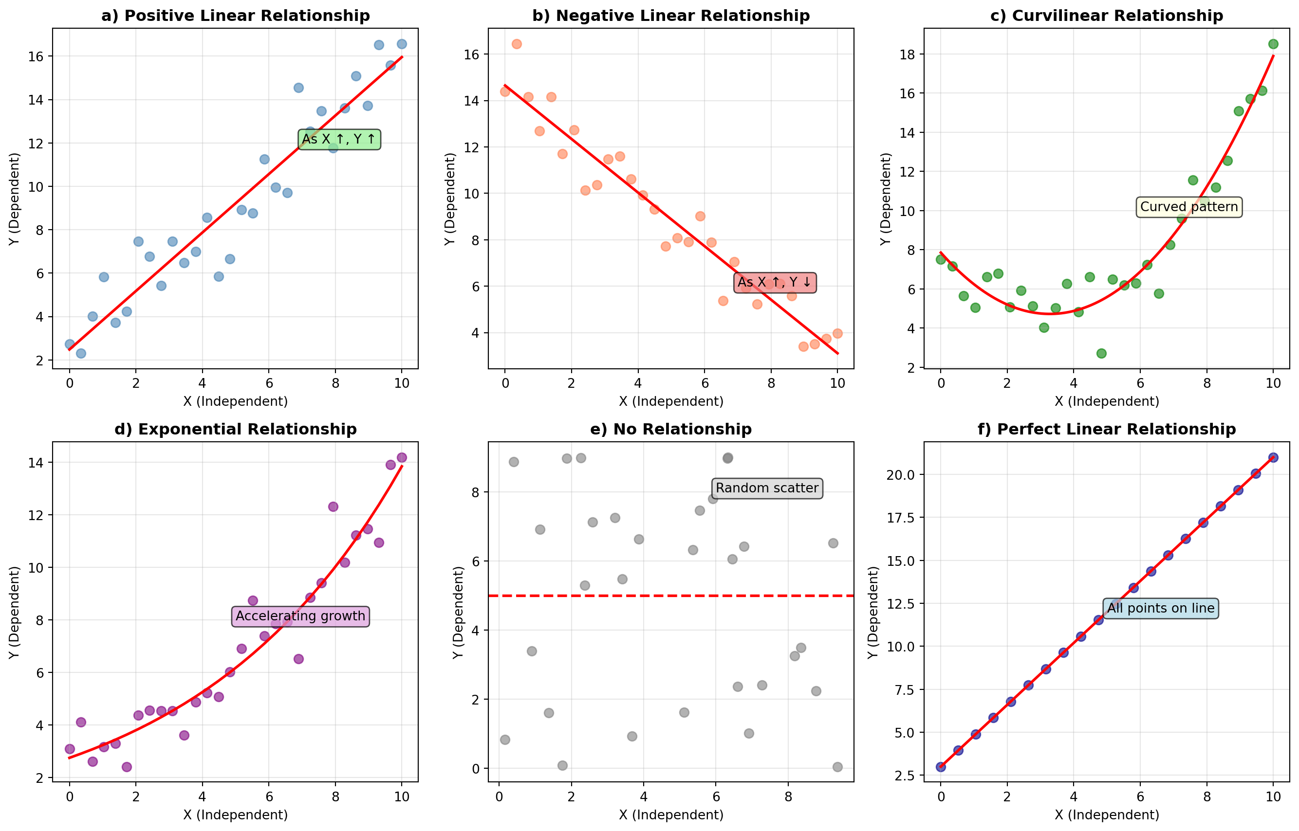
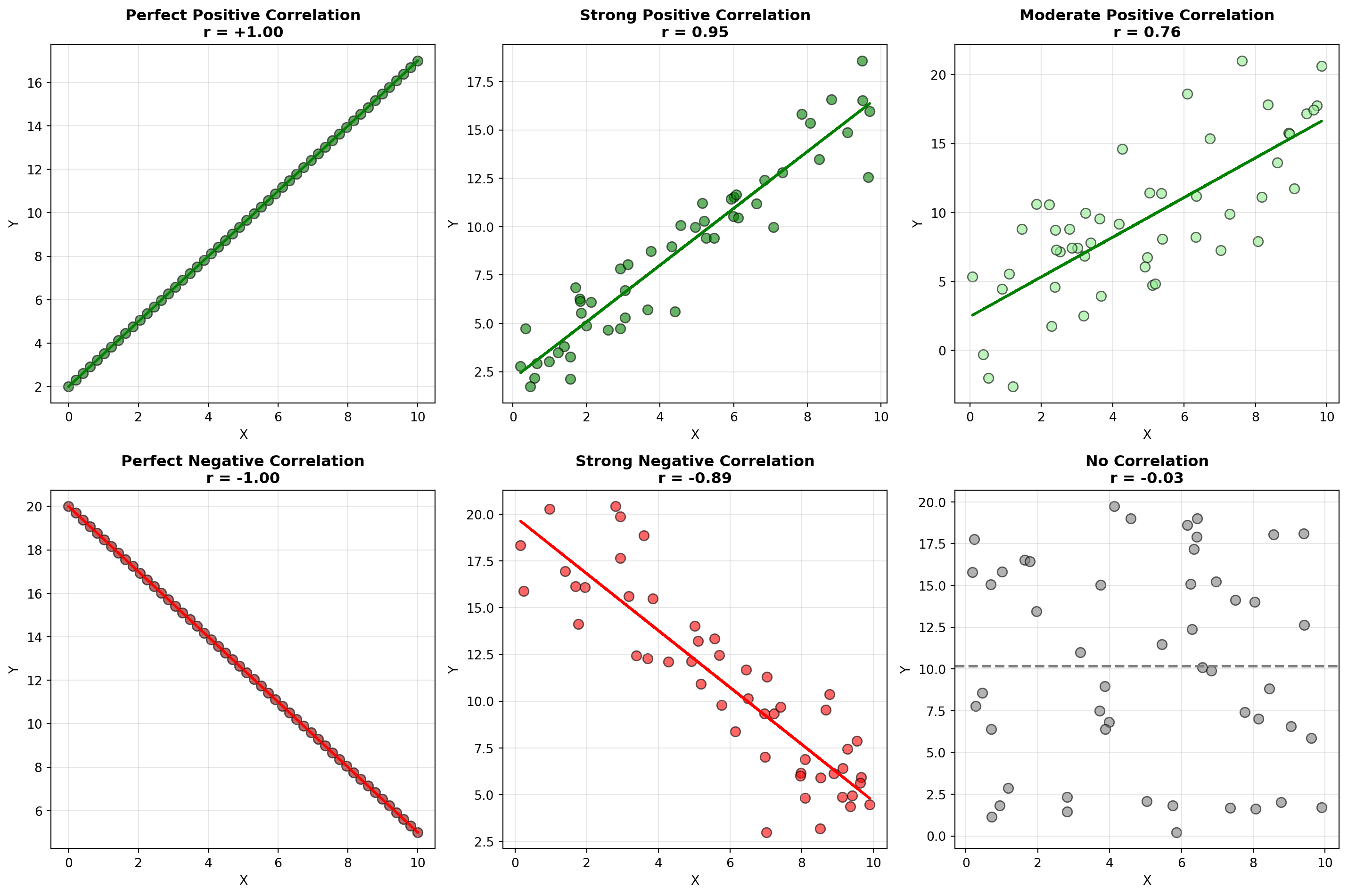
ImportantInterpreting Scatter Diagrams
- Figure a): Positive linear relationship - as X increases (decreases), Y increases (decreases)
- Figure b): Negative linear relationship - as X increases, Y decreases
- Figures c) and d): Curvilinear relationships - cannot be well described by a straight line
- Figure e): No relationship - no detectable pattern between X and Y
- Figure f): Perfect linear relationship - all points fall exactly on a line (rare in real data)
12.6 11.3 The Equation of a Straight Line
Before diving into regression analysis, let’s review the mathematical equation of a straight line. Only two points are needed to draw a straight line representing a linear relationship.
12.6.1 Basic Form
The equation of a straight line can be expressed as:
Equation of a Line
Y = b_0 + b_1 X \quad [11.1]
where: - b_0 is the intercept (where the line crosses the Y-axis) - b_1 is the slope of the line
12.6.2 Example: Understanding Slope and Intercept
Consider the equation: Y = 5 + 2X
- Intercept (b_0 = 5): The line crosses the Y-axis at 5
- Slope (b_1 = 2): The slope is calculated as:
b_1 = \text{slope} = \frac{\text{vertical change}}{\text{horizontal change}} = \frac{2}{1} = 2
This means: For every one-unit change in X, Y changes by 2 units.
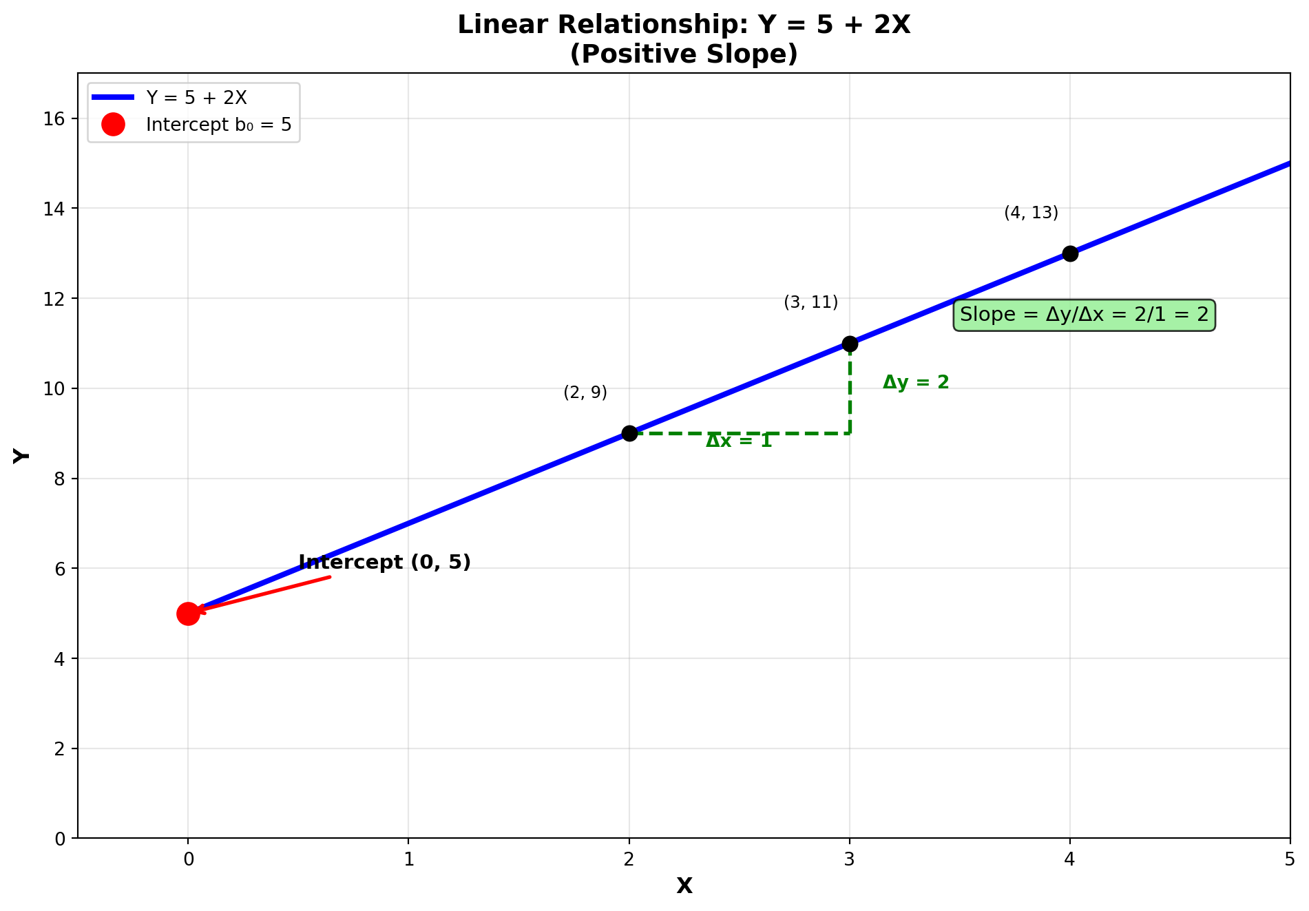
Notice that as X increases from 2 to 3 (an increase of 1 unit), Y increases from 9 to 11 (an increase of 2 units).
12.6.3 Different Slope Values
The slope b_1 determines the nature of the relationship:
- 1. Positive Slope (b_1 > 0)
- Variables move in the same direction
- Example: Y = 5 + 2X
- 2. Negative Slope (b_1 < 0)
- Variables move in opposite directions
- Example: Y = 10 - 3X
- For every one-unit increase in X, Y decreases by 3 units
- 3. Zero Slope (b_1 = 0)
- No linear relationship
- Example: Y = 10 + 0X = 10
- Changes in X have no effect on Y
12.7 11.4 Deterministic vs. Stochastic Relationships
12.7.1 Deterministic Relationships
A deterministic relationship can be expressed by a formula that provides exact conversions.
Example: Converting miles per hour (mph) to kilometers per hour (kph): 1 \text{ mph} = 1.6 \text{ kph}
Therefore: 5 \text{ mph} = 5(1.6) = 8.0 \text{ kph}
This is a deterministic model because the relationship is exact and there is no error (except for rounding).
12.7.2 Stochastic (Random) Relationships
Unfortunately, very few relationships in the business world are this exact. When using one variable to explain another, there is usually some variation in the relationship.
Example: Vita+Plus, Inc. (health product distributors) wants to develop a regression model using advertising to explain sales revenue.
They will likely find that: - When advertising is set at amount X_i, sales have value Y_i - The next time advertising is set at the same amount, sales may produce a different value - The dependent variable (sales) exhibits some degree of randomness
Therefore, there will be some error in attempting to explain or predict sales. Such a model is stochastic due to the presence of random variation:
Population (True) Regression Model
Y = \beta_0 + \beta_1 X + \varepsilon \quad [11.4]
where: - \beta_0 + \beta_1 X is the deterministic portion - \varepsilon (epsilon) is the error term (random component) - \beta_0 and \beta_1 are population parameters (usually unknown)
12.7.3 Sample-Based Estimation
The parameters \beta_0 and \beta_1 remain unknown and can only be estimated using sample data:
Sample Regression Model
Y = b_0 + b_1 X + e \quad [11.5]
where: - b_0 and b_1 are estimates of \beta_0 and \beta_1 - e is the residual (observed error in the sample)
The residual e recognizes that not all observations fall exactly on a straight line. If we knew the exact value of e, we could calculate Y precisely. However, because e is random, Y can only be estimated.
12.7.4 The Estimated Regression Model
The regression model therefore takes the form:
Estimated Regression Equation
\hat{Y} = b_0 + b_1 X \quad [11.6]
where: - \hat{Y} (read as “Y-hat”) is the estimated value of Y - b_0 is the estimated intercept - b_1 is the estimated slope
NoteNotation Summary
| Symbol | Meaning | Type |
|---|---|---|
| Y | Actual observed value | Data |
| \hat{Y} | Predicted/estimated value | Calculated from model |
| \beta_0, \beta_1 | True population parameters | Unknown |
| b_0, b_1 | Sample estimates of parameters | Calculated from data |
| \varepsilon | True population error | Unknown/theoretical |
| e | Sample residual | Calculated: e = Y - \hat{Y} |
12.8 Section Exercises
Exercise 12.1 (Understanding Regression Concepts)
- What is the difference between simple regression and multiple regression?
- What is the difference between linear regression and curvilinear regression? How does Y change when X changes in each case?
- Differentiate between the deterministic and stochastic components of a regression model.
- Why is the ordinary least squares method called “least squares”? What role does error play in this analysis?
Exercise 12.2 (Identifying Variables) Identify the dependent and independent variables in each of these cases:
- Time spent working on an assignment and the grade received
- Son’s height and father’s height
- A woman’s age and the cost of her life insurance
- Price of a product and the number of units sold
- Demand for a product and the number of consumers in the market
Exercise 12.3 (Creating Scatter Diagrams) Given the following data for X and Y:
\begin{aligned} X: & \quad 28, 54, 67, 37, 41, 69, 76 \\ Y: & \quad 14, 21, 36, 39, 18, 54, 52 \end{aligned}
- Create a scatter diagram for the data
- What do the data suggest about a relationship between X and Y?
- Draw a line to approximate the relationship
Exercise 12.4 (Regression Terminology)
- What is the difference between \hat{Y}_i and Y_i in regression analysis?
- What is the term \varepsilon in the regression model and why does it occur?
- Explain the meaning of “regression to the mean” in the historical context of Sir Francis Galton’s work
12.9 Section Summary
TipKey Takeaways
- Regression analysis studies relationships between variables to make predictions
- Dependent variable (Y): The outcome we want to explain or predict
- Independent variable (X): The predictor we use to explain Y
- Linear relationship: Y changes by a constant amount when X changes
- Scatter diagrams reveal the type and strength of relationships visually
- Stochastic models include an error term because real-world relationships aren’t perfect
- Historical origin: Sir Francis Galton developed regression studying hereditary patterns
12.10 11.5 Ordinary Least Squares: The Best-Fit Line
The purpose of regression analysis is to determine a line that fits the data better than any other line that could be drawn. To illustrate this, let’s assume that Vita+Plus, Inc. collected data on advertising expenditures and sales revenue for 5 months, as shown in Table 11.1.
Table 11.1: Sales Data for Vita+Plus, Inc.
| Month | Sales (in $1,000s) | Advertising (in $100s) |
|---|---|---|
| 1 | $450 | $50 |
| 2 | 380 | 40 |
| 3 | 540 | 65 |
| 4 | 500 | 55 |
| 5 | 420 | 45 |
Although a sample of only 5 observations would probably be insufficient in practice, it will serve our purposes for now.
12.10.1 Understanding the Error Term
These five data points and the line that best fits them appear in a scatter diagram. This line is determined by estimating b_0 and b_1. A mathematical procedure used to estimate these values is called Ordinary Least Squares (OLS).
OLS produces a line that extends through the center of the scatter plot, approximating all data points better than any other line.
For the 5 data points Y_i in the scatter diagram, these are the actual observed values for Y from Table 11.1. The values \hat{Y}_i are obtained from the regression line and represent the estimated sales.
The difference between what Y actually was (Y_i) and what we estimate it to be (\hat{Y}_i) is the error.
The Error Term
\text{Error} = (Y_i - \hat{Y}_i) \quad [11.7]
- If the actual value Y_i is greater than the estimate \hat{Y}_i, then (Y_i - \hat{Y}_i) > 0 and the error is positive (we underestimated)
- If the actual value Y_i is less than the estimate \hat{Y}_i, then (Y_i - \hat{Y}_i) < 0 and the error is negative (we overestimated)
12.10.2 The Principle of Least Squares
Because some errors are negative and some are positive, OLS produces a line such that:
Sum of Errors Equals Zero
\sum (Y_i - \hat{Y}_i) = 0
More importantly, OLS ensures that the sum of squared errors is minimized. That is, if we: 1. Take the differences (all vertical) between actual Y values and the regression line 2. Square these differences 3. Sum them
The resulting number will be smaller than what we would obtain with any other line.
OLS Minimizes Sum of Squared Errors
\sum (Y_i - \hat{Y}_i)^2 = \min \quad [11.8]
This is why it’s called Ordinary Least Squares – it produces a line such that the sum of squared errors is the minimum possible.
ImportantWhy Square the Errors?
- Eliminates sign issues: Squaring makes all values positive, preventing cancellation
- Penalizes large errors: Larger deviations are penalized more heavily
- Mathematical tractability: Squared terms have nice derivative properties for optimization
- Statistical properties: Produces unbiased estimates under certain assumptions
12.10.3 Computing Sums of Squares and Cross Products
To determine the best-fit line, OLS requires calculating:
Sum of Squares for X
SCx = \sum(X_i - \bar{X})^2 = \sum X^2 - \frac{(\sum X)^2}{n} \quad [11.9]
Sum of Squares for Y
SCy = \sum(Y_i - \bar{Y})^2 = \sum Y^2 - \frac{(\sum Y)^2}{n} \quad [11.10]
Sum of Cross Products
SCxy = \sum(X_i - \bar{X})(Y_i - \bar{Y}) = \sum XY - \frac{(\sum X)(\sum Y)}{n} \quad [11.11]
NoteComputational Forms
The first portion of each formula: - SCx = \sum(X_i - \bar{X})^2 - SCy = \sum(Y_i - \bar{Y})^2 - SCxy = \sum(X_i - \bar{X})(Y_i - \bar{Y})
illustrates how the OLS line is based on deviations from the mean. However, these are tedious to calculate manually. The second versions (computational formulas) are much easier for hand calculations.
12.10.4 Calculating the Regression Coefficients
Given the sums of squares and cross products, it’s straightforward to calculate:
The Slope (Regression Coefficient)
b_1 = \frac{SCxy}{SCx} \quad [11.12]
The Intercept (Regression Constant)
b_0 = \bar{Y} - b_1\bar{X} \quad [11.13]
where \bar{Y} and \bar{X} are the means of the Y and X values.
WarningPrecision Warning
These calculations are extremely sensitive to rounding. This is especially true for the coefficient of determination (discussed later). Therefore, it’s advisable to carry calculations to five or six decimal places for accuracy.
12.11 11.6 Example: Hop Scotch Airlines
The management of Hop Scotch Airlines, the world’s smallest carrier airline, believes there’s a direct relationship between advertising expenditures and the number of passengers who choose to fly Hop Scotch.
To determine if this relationship exists and what its exact nature might be, statisticians employed by Hop Scotch decided to use OLS procedures to determine the regression model.
Monthly values for advertising expenses and number of passengers were collected for the n = 15 most recent months. The data appear in Table 11.2, along with other necessary calculations for finding the regression model.
| Observation (Month) | Advertising (X) (in $1,000s) | Passengers (Y) (in 1,000s) | XY | X^2 | Y^2 |
|---|---|---|---|---|---|
| 1 | 10 | 15 | 150 | 100 | 225 |
| 2 | 12 | 17 | 204 | 144 | 289 |
| 3 | 8 | 13 | 104 | 64 | 169 |
| 4 | 17 | 23 | 391 | 289 | 529 |
| 5 | 10 | 16 | 160 | 100 | 256 |
| 6 | 15 | 21 | 315 | 225 | 441 |
| 7 | 10 | 14 | 140 | 100 | 196 |
| 8 | 14 | 20 | 280 | 196 | 400 |
| 9 | 19 | 24 | 456 | 361 | 576 |
| 10 | 10 | 17 | 170 | 100 | 289 |
| 11 | 11 | 16 | 176 | 121 | 256 |
| 12 | 13 | 18 | 234 | 169 | 324 |
| 13 | 16 | 23 | 368 | 256 | 529 |
| 14 | 10 | 15 | 150 | 100 | 225 |
| 15 | 12 | 16 | 192 | 144 | 256 |
| Totals | 187 | 268 | 3,490 | 2,469 | 4,960 |
12.11.1 Step-by-Step Solution
With this dataset and the calculations for XY, X^2, and Y^2, it’s easy to determine the regression model.
Step 1: Calculate Sums of Squares and Cross Products
\begin{aligned} SCx &= \sum X^2 - \frac{(\sum X)^2}{n} \\ &= 2,469 - \frac{(187)^2}{15} \\ &= 2,469 - \frac{34,969}{15} \\ &= 2,469 - 2,331.266667 \\ &= 137.733333 \end{aligned}
\begin{aligned} SCy &= \sum Y^2 - \frac{(\sum Y)^2}{n} \\ &= 4,960 - \frac{(268)^2}{15} \\ &= 4,960 - \frac{71,824}{15} \\ &= 4,960 - 4,788.266667 \\ &= 171.733333 \end{aligned}
\begin{aligned} SCxy &= \sum XY - \frac{(\sum X)(\sum Y)}{n} \\ &= 3,490 - \frac{(187)(268)}{15} \\ &= 3,490 - \frac{50,116}{15} \\ &= 3,490 - 3,341.066667 \\ &= 148.933333 \end{aligned}
Step 2: Calculate the Slope (Regression Coefficient)
\begin{aligned} b_1 &= \frac{SCxy}{SCx} \\ &= \frac{148.933333}{137.733333} \\ &= 1.081317 \approx 1.08 \end{aligned}
Step 3: Calculate the Means
\bar{Y} = \frac{\sum Y}{n} = \frac{268}{15} = 17.866667
\bar{X} = \frac{\sum X}{n} = \frac{187}{15} = 12.466667
Step 4: Calculate the Intercept
\begin{aligned} b_0 &= \bar{Y} - b_1\bar{X} \\ &= 17.866667 - 1.081317(12.466667) \\ &= 17.866667 - 13.480282 \\ &= 4.386385 \approx 4.39 \end{aligned}
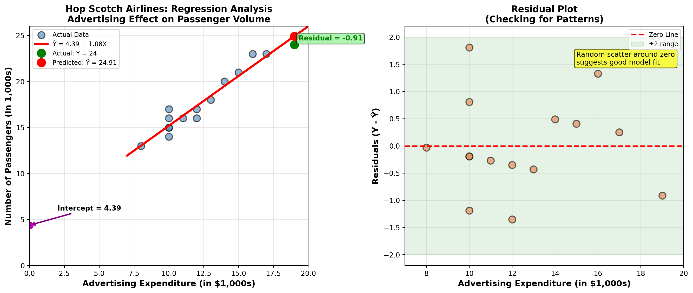
12.11.2 The Regression Model
Hop Scotch Airlines Regression Equation
\hat{Y}_i = 4.39 + 1.08X_i
where \hat{Y}_i is the predicted number of passengers (in thousands) for a given advertising expenditure X_i (in thousands).
12.11.3 Interpreting the Results
- Intercept (b_0 = 4.39)
- When advertising is zero (X = 0), the model predicts 4,390 passengers. This represents the “baseline” demand without advertising.
- Slope (b_1 = 1.08)
- For every $1,000 increase in advertising expenditure, passenger count increases by approximately 1,080 passengers (1.08 thousand).
This positive slope confirms management’s belief: advertising expenditures are positively related to passenger volume.
12.11.4 Making Predictions
Example 1: If advertising expenditure is 10,000 (X = 10$):
\hat{Y}_i = 4.39 + 1.08(10) = 4.39 + 10.8 = 15.19
Prediction: Approximately 15,190 passengers
Example 2: If advertising increases to 11,000 (X = 11$):
\hat{Y}_i = 4.39 + 1.08(11) = 4.39 + 11.88 = 16.27
Prediction: Approximately 16,270 passengers
Marginal Effect: Increasing advertising by $1,000 resulted in 16.27 - 15.19 = 1.08 thousand = 1,080 additional passengers, confirming our slope interpretation.
12.11.5 Computer Output Verification
Modern statistical software like Python produces regression output automatically. Here’s what the output would show:
Regression Equation:
PASS = 4.39 + 1.08 ADVCoefficients:
Predictor    Coef     SE Coef    t-ratio    p-value
Constant    4.3863    0.9913      4.42      0.001
ADV         1.0813    0.0773     13.99      0.000
Model Summary:
s = 0.9068 R-sq = 93.8% R-sq(adj) = 93.3%The regression line passes through the middle of the scatter plot, minimizing the sum of squared vertical distances from each point to the line.
TipBusiness Interpretation
For Hop Scotch Airlines Management:
Positive ROI on Advertising: Each $1,000 spent on advertising brings approximately 1,080 new passengers
Strong Relationship: The model explains 93.8% of the variation in passenger volume (R-sq = 93.8%)
Statistical Significance: The p-value of 0.000 for advertising indicates the relationship is highly significant
Predictive Power: Management can confidently use this model for budgeting and forecasting
Strategic Insight: Even with zero advertising, baseline demand exists (4,390 passengers), suggesting brand recognition or repeat customers
12.12 Section Exercises
Exercise 12.5 (GPA and Job Offers) The career placement center at State University wants to determine if student grade point averages (GPAs) can explain the number of job offers they receive after graduation. Data for 10 recent graduates:
| Student | 1 | 2 | 3 | 4 | 5 | 6 | 7 | 8 | 9 | 10 |
|---|---|---|---|---|---|---|---|---|---|---|
| GPA | 3.25 | 2.35 | 1.02 | 0.36 | 3.69 | 2.65 | 2.15 | 1.25 | 3.88 | 3.37 |
| Offers | 3 | 3 | 1 | 0 | 5 | 4 | 2 | 2 | 6 | 2 |
- Create a scatter diagram for the data
- Calculate and interpret the regression model. What does this model tell you about the relationship between GPA and job offers?
- If Steve has a GPA of 3.22, how many job offers do you predict he will receive?
Exercise 12.6 (Income and Consumption) An economist at the Florida Department of Human Resources is preparing a study on consumer behavior. Data were collected (in thousands of dollars) to determine if a relationship exists between consumer income and consumption levels.
| Consumer | 1 | 2 | 3 | 4 | 5 | 6 | 7 | 8 | 9 | 10 | 11 | 12 |
|---|---|---|---|---|---|---|---|---|---|---|---|---|
| Income | 24.3 | 12.5 | 31.2 | 28.0 | 35.1 | 10.5 | 23.2 | 10.0 | 8.5 | 15.9 | 14.7 | 15.0 |
| Consumption | 16.2 | 8.5 | 15.0 | 17.0 | 24.2 | 11.2 | 15.0 | 7.1 | 3.5 | 11.5 | 10.7 | 9.2 |
- Create a scatter diagram for the data
- Calculate and interpret the regression model. What does this model tell you about the relationship between consumption and income? What proportion of each additional dollar earned is spent on consumption?
- What consumption would the model predict for someone earning $27,500?
Exercise 12.7 (Interest Rates and Housing Sales) A bank in Atlanta specializing in home loans is trying to analyze the real estate market by measuring how well interest rates explain the number of houses sold in the area. Data were compiled for a 10-month period:
| Month | 1 | 2 | 3 | 4 | 5 | 6 | 7 | 8 | 9 | 10 |
|---|---|---|---|---|---|---|---|---|---|---|
| Interest | 12.3 | 10.5 | 15.6 | 9.5 | 10.5 | 9.3 | 8.7 | 14.2 | 15.2 | 12.0 |
| Houses | 196 | 285 | 125 | 225 | 248 | 303 | 265 | 102 | 105 | 114 |
- Create a scatter diagram for the data
- Calculate and interpret the regression model. What does this model tell you about the relationship between interest rates and housing sales?
- If the interest rate is 9.5%, how many houses would be sold according to the model?
Exercise 12.8 (Production Costs) Overland Group produces truck parts used in semi-trailers. The chief accountant wants to develop a regression model to predict costs. Units produced is selected as the predictor variable. Costs are in thousands of dollars, units in hundreds.
| Units | 12.3 | 8.3 | 6.5 | 4.8 | 14.6 | 14.6 | 14.6 | 6.5 |
|---|---|---|---|---|---|---|---|---|
| Cost | 6.2 | 5.3 | 4.1 | 4.4 | 5.2 | 4.8 | 5.9 | 4.2 |
- Create a scatter diagram for the data
- Calculate and interpret the regression model. What does the model tell the accountant about the relationship between production and costs?
- According to the model, how much would it cost to produce 750 units?
Exercise 12.9 (Distance and Class Absences) Professor Mundane has noticed many students have been absent from class this semester. He believes he can explain this lack of attendance by the distances students live from campus. Eleven students were surveyed about how many miles they must travel to attend class and the number of classes they’ve missed.
| Miles | 5 | 6 | 2 | 0 | 9 | 12 | 16 | 5 | 7 | 0 | 8 |
|---|---|---|---|---|---|---|---|---|---|---|---|
| Absences | 2 | 2 | 4 | 5 | 4 | 2 | 5 | 2 | 3 | 1 | 4 |
- Create a scatter diagram for the data
- Calculate and interpret the regression model. What does the professor discover?
- How many classes would you miss if you lived 3.2 miles from campus, according to the model?
Exercise 12.10 (Employment Test Scores and Performance Ratings) The personnel director at Bupkus, Inc. obtained data on 100 employees regarding entrance tests administered at hiring and subsequent ratings employees received from supervisors one year later. Test scores ranged from 0 to 10, and ratings used a 5-point system. The director wants to use the regression model to predict rating (R) based on test score (S). The results are:
\begin{aligned} \sum S &= 522 \quad \sum R = 326 \quad \sum SR = 17,325 \\ \sum S^2 &= 28,854 \quad \sum R^2 = 10,781 \end{aligned}
Develop and interpret the regression model. What can the director predict about the rating of an employee who scored 7 on the test?
NoteNote for Students
Keep your calculations from exercises 1-6 for use throughout the rest of this chapter. Using the same data, you will avoid having to recalculate SCx, SCy, and SCxy each time. You will gain additional experience with other problems at the end of the chapter.
12.13 Section Summary
TipKey Takeaways: Ordinary Least Squares
- OLS minimizes the sum of squared vertical distances from data points to the regression line
- Regression slope (b_1): Measures the change in Y for each one-unit change in X
- Regression intercept (b_0): The predicted value of Y when X = 0
- Computational formulas make hand calculations manageable
- Precision matters: Carry calculations to 5-6 decimal places to avoid rounding errors
- Residuals: The differences between actual and predicted values reveal model fit
- Business value: Regression provides quantitative relationships for decision-making
12.14 11.7 Standard Error of Estimation
Now that we have a regression model, the next logical question is: How good is it? How well does the model fit the data? The standard error of estimation provides a critical measure of this goodness of fit.
12.14.1 Defining the Standard Error
The standard error of estimation, denoted S_e, measures the typical distance that observed data points fall from the regression line. It’s conceptually similar to the standard deviation, but instead of measuring dispersion around the mean of a single variable, it measures dispersion around the regression line.
Standard Error of Estimation (Conceptual Form)
S_e = \sqrt{\frac{\sum(Y_i - \hat{Y}_i)^2}{n-2}} \quad [11.14]
where: - Y_i = actual observed value - \hat{Y}_i = predicted value from regression line - n - 2 = degrees of freedom (we lose 2 degrees because we estimate b_0 and b_1)
NoteWhy n-2 Degrees of Freedom?
In regression analysis, we estimate two parameters: the intercept (b_0) and the slope (b_1). Each parameter estimated “uses up” one degree of freedom from our sample of n observations, leaving us with n - 2 degrees of freedom for the error term.
12.14.2 Computational Formula
While the conceptual formula clearly shows what S_e measures, it’s tedious to calculate manually because we’d need to: 1. Calculate \hat{Y}_i for each observation 2. Find each difference (Y_i - \hat{Y}_i) 3. Square each difference 4. Sum all squared differences
A more efficient computational approach uses the sum of squared errors (SCE) and mean squared error (CME):
Sum of Squared Errors
SCE = SCy - \frac{(SCxy)^2}{SCx} \quad [11.15]
Mean Squared Error (CME)
CME = \frac{SCE}{n-2} \quad [11.16]
Standard Error of Estimation (Computational Form)
S_e = \sqrt{CME} \quad [11.17]
12.14.3 Application to Hop Scotch Airlines
Let’s calculate the standard error for the Hop Scotch Airlines example, where: - SCy = 171.733333 - SCxy = 148.933333 - SCx = 137.733333 - n = 15
Step 1: Calculate SCE
\begin{aligned} SCE &= SCy - \frac{(SCxy)^2}{SCx} \\ &= 171.733333 - \frac{(148.933333)^2}{137.733333} \\ &= 171.733333 - \frac{22,181.14}{137.733333} \\ &= 171.733333 - 161.044 \\ &= 10.6893 \end{aligned}
Step 2: Calculate CME
\begin{aligned} CME &= \frac{SCE}{n-2} \\ &= \frac{10.6893}{15-2} \\ &= \frac{10.6893}{13} \\ &= 0.82226 \end{aligned}
Step 3: Calculate S_e
\begin{aligned} S_e &= \sqrt{CME} \\ &= \sqrt{0.82226} \\ &= 0.90678 \approx 0.907 \end{aligned}
12.14.4 Interpreting the Standard Error
The standard error is always expressed in the same units as the dependent variable Y. For Hop Scotch Airlines:
S_e = 0.907 thousand passengers = 907 passengers
This means that the typical prediction error is about 907 passengers. The actual number of passengers typically deviates from the regression line prediction by approximately 907 passengers.
12.14.5 The Empirical Rule Applied to Regression
Just as the empirical rule applies to standard deviation for a single variable, it applies to the standard error in regression analysis:
ImportantEmpirical Rule for Regression
If the errors are normally distributed:
- 68.3% of observations fall within \pm 1S_e of the regression line
- 95.5% of observations fall within \pm 2S_e of the regression line
- 99.7% of observations fall within \pm 3S_e of the regression line
12.14.6 Practical Application
Let’s apply this to a specific prediction. When advertising expenditure is X = 10 thousand dollars:
\hat{Y}_i = 4.39 + 1.08(10) = 15.19 \text{ thousand passengers}
This represents the average number of passengers we’d expect when X = 10.
One Standard Error Band: - Upper bound: 15.19 + 0.907 = 16.10 thousand (16,100 passengers) - Lower bound: 15.19 - 0.907 = 14.29 thousand (14,290 passengers)
Interpretation: When Hop Scotch spends $10,000 on advertising: - 68.3% of the time, passenger count will be between 14,290 and 16,100 - 31.7% of the time, passenger count will fall outside this range (either below 14,290 or above 16,100)
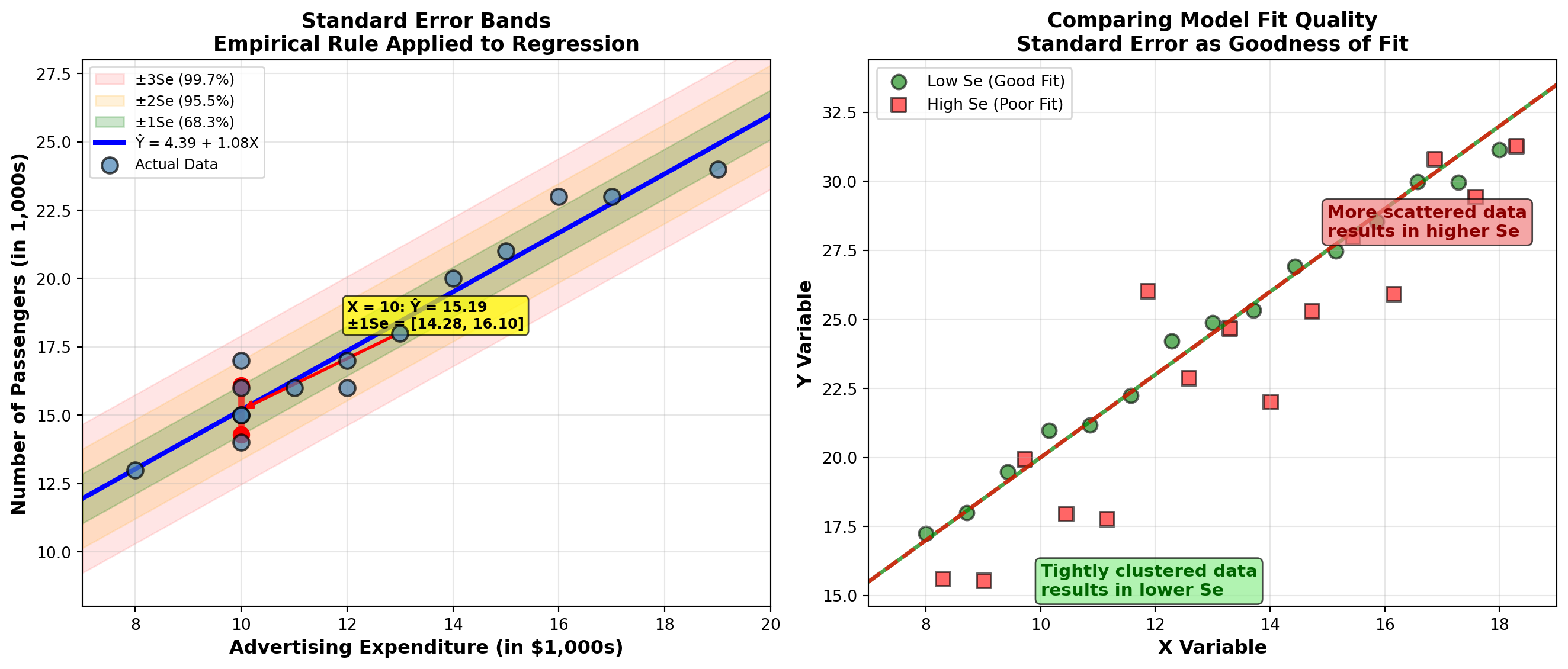
12.14.7 Standard Error as a Goodness-of-Fit Measure
The standard error provides a quantifiable measure of how well the regression model fits the data:
- Smaller S_e → Better Fit
- Data points cluster tightly around the regression line. Predictions are more accurate.
- Larger S_e → Poorer Fit
- Data points are more scattered around the regression line. Predictions are less reliable.
As shown in the visualization above: - When data are tightly clustered around the line, S_e is small (good fit) - When data are widely dispersed, S_e is large (poor fit)
WarningContext Matters for Interpretation
Whether S_e = 0.907 represents a “good” or “poor” fit depends on context:
- For Hop Scotch: A typical error of 907 passengers might be acceptable given that monthly passenger volumes range from 13,000 to 24,000
- Relative measure: Compare S_e to the range of Y values. Here, the range is (24 - 13) = 11 thousand, so S_e = 0.907 is about 8% of the range
- Business decision: Is this level of prediction accuracy sufficient for planning purposes?
12.14.8 Verification with Computer Output
From the Python output shown earlier:
s = 0.9068 R-sq = 93.8% R-sq(adj) = 93.3%The computer-calculated standard error (s = 0.9068) matches our hand calculation (S_e = 0.907), confirming our work.
12.15 Section Exercises
Exercise 12.11 (Standard Error for State University) Using your calculations from the GPA and job offers exercise (Exercise 9), calculate and interpret the standard error of estimation for State University. Create a graph illustrating the interpretation. How can this be used as a measure of goodness of fit?
Exercise 12.12 (Standard Error for Florida Department of Human Resources) Based on the data from the income and consumption exercise (Exercise 10), what is the standard error of estimation for the Florida Department of Human Resources? How would you interpret the results? Use a graph in your interpretation.
Exercise 12.13 (Standard Error for Atlanta Bank) Calculate and interpret the standard error of estimation for the interest rates and housing sales exercise (Exercise 11) about the Atlanta bank.
Exercise 12.14 (Standard Error for Overland Group) The Overland Group from the production costs exercise (Exercise 12) now wants to know the standard error of estimation for their cost prediction model.
Exercise 12.15 (Standard Error for Professor Mundane) What is the standard error of estimation that Professor Mundane will experience in the distance and absences exercise (Exercise 13)?
12.16 11.8 Correlation Analysis: Measuring Relationship Strength
The regression model has provided a clear picture of the relationship between Hop Scotch Airlines’ advertising expenditures and the number of brave travelers who line up at the ticket counter. The positive value for b_1 indicates a direct relationship: as advertising increases, so does the number of passengers.
Now it’s useful to obtain a measure of the strength of that relationship. This is the function of the correlation coefficient, developed by Carl Pearson at the end of the 19th century. Sometimes called the Pearson product-moment correlation coefficient, it’s represented by r.
12.16.1 The Correlation Coefficient
Range of the Correlation Coefficient
-1 \leq r \leq +1 \quad [11.18]
The correlation coefficient can assume any value between -1 and +1:
- r = -1 (Perfect Negative Correlation)
- All observations fall on a straight line with negative slope. X and Y move in opposite directions perfectly.
- r = 0 (No Linear Correlation)
- No linear relationship exists between X and Y. Knowing X provides no information about Y.
- r = +1 (Perfect Positive Correlation)
- All observations fall on a straight line with positive slope. X and Y move in the same direction perfectly.
- -1 < r < 0 (Negative Correlation)
- X and Y tend to move in opposite directions, but the relationship isn’t perfect.
- 0 < r < +1 (Positive Correlation)
- X and Y tend to move in the same direction, but the relationship isn’t perfect.
TipInterpreting Correlation Strength
General guidelines (though context-dependent):
- |r| \geq 0.9: Very strong relationship
- 0.7 \leq |r| < 0.9: Strong relationship
- 0.5 \leq |r| < 0.7: Moderate relationship
- 0.3 \leq |r| < 0.5: Weak relationship
- |r| < 0.3: Very weak or no relationship
The closer |r| is to 1, the stronger the linear relationship.
12.16.2 Understanding What r Measures
To fully understand what the correlation coefficient measures, we need to develop three measures of deviation. Consider observation 13 from the Hop Scotch data (where X = 16 and Y = 23):
- Total Deviation of Y
- The amount by which individual Y values vary from their mean \bar{Y}:
(Y_i - \bar{Y}) = 23 - 17.87 = 5.13
- Explained Deviation
- The difference between what the regression model predicts (\hat{Y}_i) and the mean value of Y (\bar{Y}):
(\hat{Y}_i - \bar{Y}) = 21.68 - 17.87 = 3.81
where \hat{Y}_i = 4.39 + 1.08(16) = 21.68
- Unexplained Deviation (Residual)
- The portion of total deviation that is NOT explained by the regression model (the error):
(Y_i - \hat{Y}_i) = 23 - 21.68 = 1.32
Fundamental Relationship:
\text{Total Deviation} = \text{Explained Deviation} + \text{Unexplained Deviation}
(Y_i - \bar{Y}) = (\hat{Y}_i - \bar{Y}) + (Y_i - \hat{Y}_i)
12.16.3 Sums of Squares Decomposition
When we square these deviations and sum across all observations, we get:
Sum of Squares Total (SCT)
SCT = \sum(Y_i - \bar{Y})^2 \quad [11.19]
Measures total variation in Y around its mean.
Sum of Squares Regression (SCR)
SCR = \sum(\hat{Y}_i - \bar{Y})^2 \quad [11.20]
Measures variation explained by the regression model.
Sum of Squares Error (SCE)
SCE = \sum(Y_i - \hat{Y}_i)^2 \quad [11.21]
Measures variation NOT explained by the model (residual variation).
Fundamental ANOVA Identity:
SCT = SCR + SCE
12.16.4 Calculating the Correlation Coefficient
The correlation coefficient compares explained variation to total variation:
Correlation Coefficient (Conceptual)
r = \sqrt{\frac{\text{Explained Variation}}{\text{Total Variation}}} = \sqrt{\frac{SCR}{SCT}} \quad [11.22]
However, this formula is difficult to calculate manually. A more convenient computational formula is:
Correlation Coefficient (Computational Form)
r = \frac{SCxy}{\sqrt{(SCx)(SCy)}} \quad [11.23]
This formula uses the sums of squares we’ve already calculated for the regression coefficients!
12.16.5 Application to Hop Scotch Airlines
For the Hop Scotch example: - SCxy = 148.933333 - SCx = 137.733333 - SCy = 171.733333
\begin{aligned} r &= \frac{SCxy}{\sqrt{(SCx)(SCy)}} \\ &= \frac{148.933333}{\sqrt{(137.733333)(171.733333)}} \\ &= \frac{148.933333}{\sqrt{23,654.60}} \\ &= \frac{148.933333}{153.807} \\ &= 0.9683 \end{aligned}
Interpretation: r = 0.9683 indicates a very strong positive relationship between advertising expenditures and passenger volume. When advertising increases, passengers almost always increase proportionally.
12.17 11.9 Coefficient of Determination (r^2)
Perhaps the most important measure of goodness of fit is the coefficient of determination, denoted r^2.
12.17.1 Definition and Calculation
Coefficient of Determination (Conceptual)
r^2 = \frac{\text{Explained Variation}}{\text{Total Variation}} = \frac{SCR}{SCT} \quad [11.24]
Computational Formula
r^2 = \frac{(SCxy)^2}{(SCx)(SCy)} \quad [11.25]
Or simply:
r^2 = (r)^2
Square the correlation coefficient!
12.17.2 Application to Hop Scotch Airlines
Method 1: Using the formula
\begin{aligned} r^2 &= \frac{(SCxy)^2}{(SCx)(SCy)} \\ &= \frac{(148.933333)^2}{(137.733333)(171.733333)} \\ &= \frac{22,181.14}{23,654.60} \\ &= 0.93776 \approx 0.938 \end{aligned}
Method 2: Squaring the correlation coefficient
r^2 = (0.9683)^2 = 0.9376 \approx 0.938
Both methods give us r^2 = 0.938 or 93.8%.
12.17.3 Interpreting r^2
The coefficient of determination reveals what percentage of the change in Y is explained by the change in X.
For Hop Scotch Airlines:
ImportantBusiness Interpretation of r^2 = 0.938
93.8% of the variation in passenger volume is explained by advertising expenditure.
This means: - 93.8% of the changes in passenger numbers can be attributed to changes in advertising spending - 6.2% of passenger variation is due to other factors (e.g., seasonality, competitors, economic conditions, random variation) - The regression model captures nearly all the systematic variation in the data
This high r^2 indicates an excellent fit. The model is highly effective for prediction and decision-making.
12.17.4 Important Cautions About r^2
WarningCritical Limitations of r^2
Linear Relationships Only: r^2 measures only linear relationships. Two variables can have r^2 = 0 yet still be strongly related in a curvilinear way.
Correlation ≠ Causation: The 93.8% does NOT mean advertising causes 93.8% of the passenger changes. It only means they are associated.
Context Dependent: What constitutes a “good” r^2 varies by field:
- Physical sciences: Often expect r^2 > 0.95
- Social sciences: r^2 > 0.60 may be considered strong
- Business/economics: r^2 > 0.70 typically indicates good fit
Sample Size Matters: With very large samples, even weak relationships can yield statistically significant r^2 values
12.17.5 Computer Output Verification
From the Python output shown earlier:
s = 0.9068 R-sq = 93.8% R-sq(adj) = 93.3%The computer-calculated r^2 = 93.8\% matches our hand calculation exactly!
Note: “R-sq(adj)” is the adjusted r^2, which adjusts for the number of predictors in the model. This becomes important in multiple regression (Chapter 12).
12.18 Section Exercises
Exercise 12.16 (Coefficient of Determination as Goodness of Fit) How can the coefficient of determination be used as a measure of goodness of fit? Create a graph to illustrate your explanation.
Exercise 12.17 (GPA and Job Offers Correlation) What is the strength of the relationship between GPA and job offers in Exercise 9? Calculate and interpret both r and r^2.
Exercise 12.18 (Income and Consumption Correlation) Calculate and interpret the correlation coefficient and coefficient of determination for the Florida Department of Human Resources data in Exercise 10.
Exercise 12.19 (Housing Sales Explained by Interest Rates) How much of the change in houses sold can be explained by the interest rate in Exercise 11? What does this tell you about the strength of the relationship?
Exercise 12.20 (Professor Mundane’s Model Strength) What is the strength of Professor Mundane’s model used in Exercise 13 to explain student absences? How much of the variation in absences is explained by distance from campus?
12.19 Section Summary
TipKey Takeaways: Model Evaluation
Standard Error of Estimation (S_e): - Measures typical prediction error in the same units as Y - Smaller S_e indicates better fit - Can be interpreted using the empirical rule (68%-95%-99.7%) - Provides absolute measure of scatter around regression line
Correlation Coefficient (r): - Measures strength and direction of linear relationship - Range: -1 \leq r \leq +1 - Sign indicates direction (positive/negative) - Magnitude indicates strength (closer to ±1 is stronger)
Coefficient of Determination (r^2): - Most important goodness-of-fit measure - Percentage of variation in Y explained by X - Range: 0 \leq r^2 \leq 1 (often expressed as percentage) - Higher r^2 means better predictive power - Remember: Correlation does NOT imply causation!
For Hop Scotch Airlines: - S_e = 0.907 (typical error of 907 passengers) - r = 0.9683 (very strong positive relationship) - r^2 = 0.938 (93.8% of passenger variation explained) - Conclusion: Excellent model for business decision-making
12.20 11.10 Hypothesis Testing for Regression Parameters
The statistical results suggest a relationship between passengers and advertising for Hop Scotch Airlines. The non-zero values for the regression coefficient (b_1 = 1.08) and correlation coefficient (r = 0.968) indicate that as advertising expenditures change, the number of passengers changes.
However, these results are based on a sample of only n = 15 observations. As always, we must ask: Does a relationship exist at the population level? It could be that due to sampling error, the population parameters are actually zero. We must test the population parameters to ensure that our sample findings differ significantly from zero.
12.20.1 A. Testing the Regression Slope (\beta_1)
If the slope of the true but unknown population regression line is zero, there is no relationship between passengers and advertising—contrary to our sample results.
If we were to create a scatter diagram for the population of all possible (X, Y) data points, it might look like the figure below, showing no pattern. When collecting our sample, we might have included only 15 observations from within a particular region that falsely suggests a positive relationship.
We must test the hypothesis:
\begin{aligned} H_0: \beta_1 &= 0 \quad \text{(No relationship)} \\ H_A: \beta_1 &\neq 0 \quad \text{(Relationship exists)} \end{aligned}
The t-Test for the Regression Coefficient
t = \frac{b_1 - \beta_1}{S_{b_1}} \quad [11.26]
with n - 2 degrees of freedom.
where S_{b_1} is the standard error of the regression coefficient, which recognizes that different samples produce different values for b_1.
Standard Error of the Regression Coefficient
S_{b_1} = \frac{S_e}{\sqrt{SCx}} \quad [11.27]
NoteWhy Does b_1 Have Sampling Variability?
If we took different samples of n = 15 months and calculated a regression equation for each, we’d likely get different values for b_0 and b_1 each time. The standard error S_{b_1} measures this sampling variability in the slope estimate.
If \beta_1 = 0 in the population, the sample values b_1 would be distributed around zero as shown below.
12.20.2 Application to Hop Scotch Airlines
Step 1: Calculate the Standard Error
Given: - S_e = 0.907 - SCx = 137.733333
\begin{aligned} S_{b_1} &= \frac{S_e}{\sqrt{SCx}} \\ &= \frac{0.907}{\sqrt{137.733333}} \\ &= \frac{0.907}{11.735} \\ &= 0.07726 \end{aligned}
Step 2: Calculate the Test Statistic
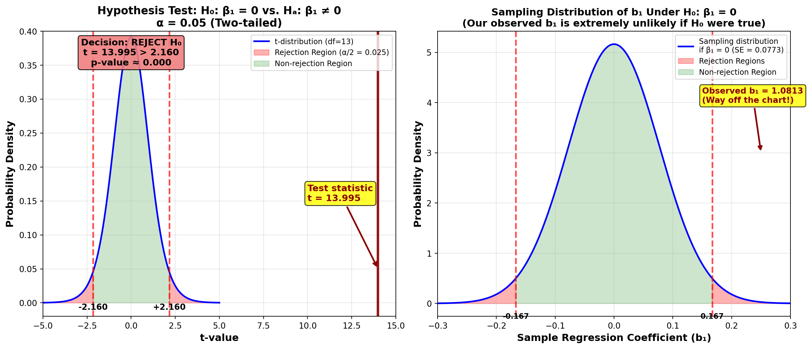
\begin{aligned} t &= \frac{b_1 - \beta_1}{S_{b_1}} \\ &= \frac{1.0813 - 0}{0.07726} \\ &= 13.995 \end{aligned}
Step 3: Determine the Critical Value
For \alpha = 0.05 (5% significance level) with n - 2 = 15 - 2 = 13 degrees of freedom:
t_{0.025, 13} = \pm 2.160
(Two-tailed test, so we split \alpha in half)
Step 4: Make Decision
Decision Rule: Do not reject H_0 if t is between \pm 2.160; otherwise reject H_0.
Conclusion: Since t = 13.995 > 2.160, we reject the null hypothesis. At the 5% significance level, there appears to be a significant relationship between passengers and advertising.
This is confirmed by the Python output (shown earlier), which reports a p-value of 0.000, indicating extremely strong evidence against H_0.
ImportantWhat If We Fail to Reject H_0?
If we had not rejected the null hypothesis, we would conclude that advertising and passengers are not significantly related. In that case, we would discard this model and use a different explanatory variable instead of advertising.
Since we did reject H_0, we have strong evidence that the relationship is real (not due to chance), and advertising is a useful predictor of passenger volume.
12.20.3 Confidence Interval for \beta_1
Since we’ve rejected the hypothesis that \beta_1 = 0, the natural question is: “What IS its value?”
We can answer this by calculating a confidence interval for \beta_1:
Confidence Interval for the Regression Slope
\text{C.I. for } \beta_1 = b_1 \pm t_{\alpha/2, n-2} \cdot S_{b_1} \quad [11.28]
For a 95% Confidence Level:
\begin{aligned} \text{C.I. for } \beta_1 &= 1.08 \pm (2.160)(0.07726) \\ &= 1.08 \pm 0.167 \\ 0.913 &\leq \beta_1 \leq 1.247 \end{aligned}
Interpretation: We can be 95% confident that the true population regression coefficient is between 0.913 and 1.247. This means each $1,000 increase in advertising expenditure increases passenger volume by somewhere between 913 and 1,247 passengers.
12.20.4 B. Testing the Correlation Coefficient (\rho)
Much of the work done for testing the regression coefficient can be applied to testing the correlation coefficient. The purpose and rationale are very similar.
Since our correlation analysis is based on sample data, sampling error might lead to inappropriate conclusions. The sample data produced a non-zero correlation coefficient of r = 0.9683, but this could be due to sampling error. Perhaps the population correlation is actually zero, and a misleading sample caused us to assume a relationship incorrectly.
Therefore, we must test:
\begin{aligned} H_0: \rho &= 0 \quad \text{(No correlation in population)} \\ H_A: \rho &\neq 0 \quad \text{(Correlation exists in population)} \end{aligned}
where \rho (Greek letter rho) is the population correlation coefficient.
The t-Test for the Correlation Coefficient
t = \frac{r - \rho}{S_r} \quad [11.29]
where S_r is the standard error of the correlation coefficient.
Standard Error of the Correlation Coefficient
S_r = \sqrt{\frac{1 - r^2}{n - 2}} \quad [11.30]
12.20.5 Application to Hop Scotch Airlines
Step 1: Calculate the Standard Error
\begin{aligned} S_r &= \sqrt{\frac{1 - r^2}{n - 2}} \\ &= \sqrt{\frac{1 - 0.93776}{15 - 2}} \\ &= \sqrt{\frac{0.06224}{13}} \\ &= \sqrt{0.004787} \\ &= 0.0692 \end{aligned}
Step 2: Calculate the Test Statistic
\begin{aligned} t &= \frac{r - \rho}{S_r} \\ &= \frac{0.9683 - 0}{0.0692} \\ &= 13.995 \end{aligned}
Step 3: Decision
Using \alpha = 0.05 with df = 13: Critical value t_{0.025, 13} = \pm 2.160
Decision Rule: Do not reject if t is between \pm 2.160; otherwise reject.
Conclusion: Since t = 13.995 > 2.160, we reject the null hypothesis. At the 5% significance level, we conclude that the population correlation coefficient is not zero—passengers and advertising are significantly correlated.
TipImportant Observation: t Values Are Identical!
Notice that the t-value of 13.995 is the same for both: - Testing \beta_1 = 0 - Testing \rho = 0
This is not a coincidence. In simple linear regression (one predictor), these two tests are mathematically equivalent. They will always give identical results.
However, in multiple regression (Chapter 12), this equivalence does not hold. That’s why it’s important to become familiar with both tests.
12.20.6 Equivalence of the Two Tests
For simple linear regression:
F = t^2
Also: - Testing H_0: \beta_1 = 0 is equivalent to testing H_0: \rho = 0 - Both test whether there’s a significant linear relationship between X and Y
12.21 11.11 Confidence and Prediction Intervals
Regression analysis can forecast and predict values for the dependent variable. Once we’ve determined the regression equation, we can develop a point estimate for the dependent variable by substituting a given value for X and solving for Y.
However, as we’ve seen throughout this textbook, interval estimates are often preferred over point estimates. There are at least two types of interval estimates commonly used in regression:
- Confidence Interval for the Mean \mu_{Y|X}: The average value of Y for all cases where X equals a specific value
- Prediction Interval for an Individual Y_X: A single value of Y when X equals a specific value
12.21.1 A. Confidence Interval for the Mean of Y Conditional on X
Suppose we want to develop an interval estimate for the conditional mean of Y, denoted \mu_{Y|X}. This is the population mean for all values of Y, given that X equals a specific value.
Example: If X = 10 (advertising = $10,000) many times, we’d obtain many different values of Y (passenger counts). The interval we’re calculating estimates the mean of all those Y values.
Two Interpretations (for a 95% confidence interval):
First interpretation: If we set X equal to the same amount many times, we’d obtain many different values of Y. We can be 95% confident that the mean of those Y values (\mu_{Y|X}) will fall within the specified interval.
Second interpretation: If we took many samples of (X, Y) values and constructed a confidence interval based on each sample, 95% of them would contain the true mean value \mu_{Y|X}.
To calculate this interval, we must first determine S_{\hat{Y}}, the standard error of the conditional mean.
Standard Error of the Conditional Mean
S_{\hat{Y}} = S_e \sqrt{\frac{1}{n} + \frac{(X_i - \bar{X})^2}{SCx}} \quad [11.31]
where: - S_e = standard error of estimation - X_i = the given value for the independent variable - \bar{X} = mean of X values in the sample - SCx = sum of squares for X
The confidence interval for the conditional mean is:
Confidence Interval for \mu_{Y|X}
\text{C.I. for } \mu_{Y|X} = \hat{Y}_i \pm t_{\alpha/2, n-2} \cdot S_{\hat{Y}} \quad [11.32]
where \hat{Y}_i is the point estimate from the regression equation.
12.21.2 Application: Hop Scotch Airlines (Confidence Interval)
Question: What is the average passenger count when advertising = $10,000?
Given: - X_i = 10 - \bar{X} = 12.47 - S_e = 0.907 - SCx = 137.733333 - n = 15
Step 1: Calculate Standard Error of the Mean
\begin{aligned} S_{\hat{Y}} &= S_e \sqrt{\frac{1}{n} + \frac{(X_i - \bar{X})^2}{SCx}} \\ &= 0.907 \sqrt{\frac{1}{15} + \frac{(10 - 12.47)^2}{137.733333}} \\ &= 0.907 \sqrt{0.06667 + \frac{6.1009}{137.733333}} \\ &= 0.907 \sqrt{0.06667 + 0.04430} \\ &= 0.907 \sqrt{0.11097} \\ &= 0.907(0.3331) \\ &= 0.302 \end{aligned}
Step 2: Calculate Point Estimate
\hat{Y}_i = 4.39 + 1.08(10) = 15.19
Step 3: Construct 95% Confidence Interval
For 95% confidence with df = 13: t_{0.025, 13} = 2.160
\begin{aligned} \text{C.I. for } \mu_{Y|X} &= 15.19 \pm (2.160)(0.302) \\ &= 15.19 \pm 0.652 \\ 14.54 &\leq \mu_{Y|X} \leq 15.84 \end{aligned}
Interpretation: Hop Scotch can be 95% confident that if they spend $10,000 on advertising many times, the average passenger count across all those occasions will be between 14,540 and 15,840 passengers.
12.21.3 B. Prediction Interval for a Single Value of Y
The confidence interval developed above estimates the mean of all Y values when X equals a given amount. Often, it’s more useful to construct an interval for a single value of Y obtained when X is set to a given value just once.
Example: Hop Scotch might be interested in predicting the number of customers next month if they invest $10,000 in advertising. This differs from predicting the average across many months.
Key Insight: Individual values are more dispersed than means. Means tend to cluster around the center of the data, making them easier to predict. Individual values scatter more widely, making them harder to predict.
Therefore, a 95% confidence interval for a single value of Y must be wider than the interval for the conditional mean.
Two Interpretations (for a 95% prediction interval):
First interpretation: If we set X equal to some amount just once, we’ll obtain a single resulting value of Y. We can be 95% confident that this single value of Y falls within the specified interval.
Second interpretation: If we took many samples and used each to construct a prediction interval, 95% of them would contain the true value for Y.
To calculate the prediction interval, we need the standard error of the forecast, S_{Y_X}.
Standard Error of the Forecast
S_{Y_X} = S_e \sqrt{1 + \frac{1}{n} + \frac{(X_i - \bar{X})^2}{SCx}} \quad [11.33]
Notice the extra “1” under the square root compared to formula [11.31]. This accounts for the additional variability of individual values versus means.
Prediction Interval for Y_X
\text{P.I. for } Y_X = \hat{Y}_i \pm t_{\alpha/2, n-2} \cdot S_{Y_X} \quad [11.34]
12.21.4 Application: Hop Scotch Airlines (Prediction Interval)
Question: What will passenger count be next month if advertising = $10,000?
Step 1: Calculate Standard Error of the Forecast
\begin{aligned} S_{Y_X} &= S_e \sqrt{1 + \frac{1}{n} + \frac{(X_i - \bar{X})^2}{SCx}} \\ &= 0.907 \sqrt{1 + \frac{1}{15} + \frac{(10 - 12.47)^2}{137.733333}} \\ &= 0.907 \sqrt{1 + 0.06667 + 0.04430} \\ &= 0.907 \sqrt{1.11097} \\ &= 0.907(1.054) \\ &= 0.956 \end{aligned}
Step 2: Construct 95% Prediction Interval
\begin{aligned} \text{P.I. for } Y_X &= 15.19 \pm (2.160)(0.956) \\ &= 15.19 \pm 2.065 \\ 13.13 &\leq Y_X \leq 17.26 \end{aligned}
Interpretation: Hop Scotch can be 95% confident that if they spend $10,000 on advertising next month, the passenger count for that specific month will be between 13,130 and 17,260 passengers.
12.21.5 Comparing the Two Intervals
For X = 10: - Confidence interval for mean: [14.54, 15.84] (width = 1.30) - Prediction interval for individual: [13.13, 17.26] (width = 4.13)
The prediction interval is much wider because individual values are less predictable than means!
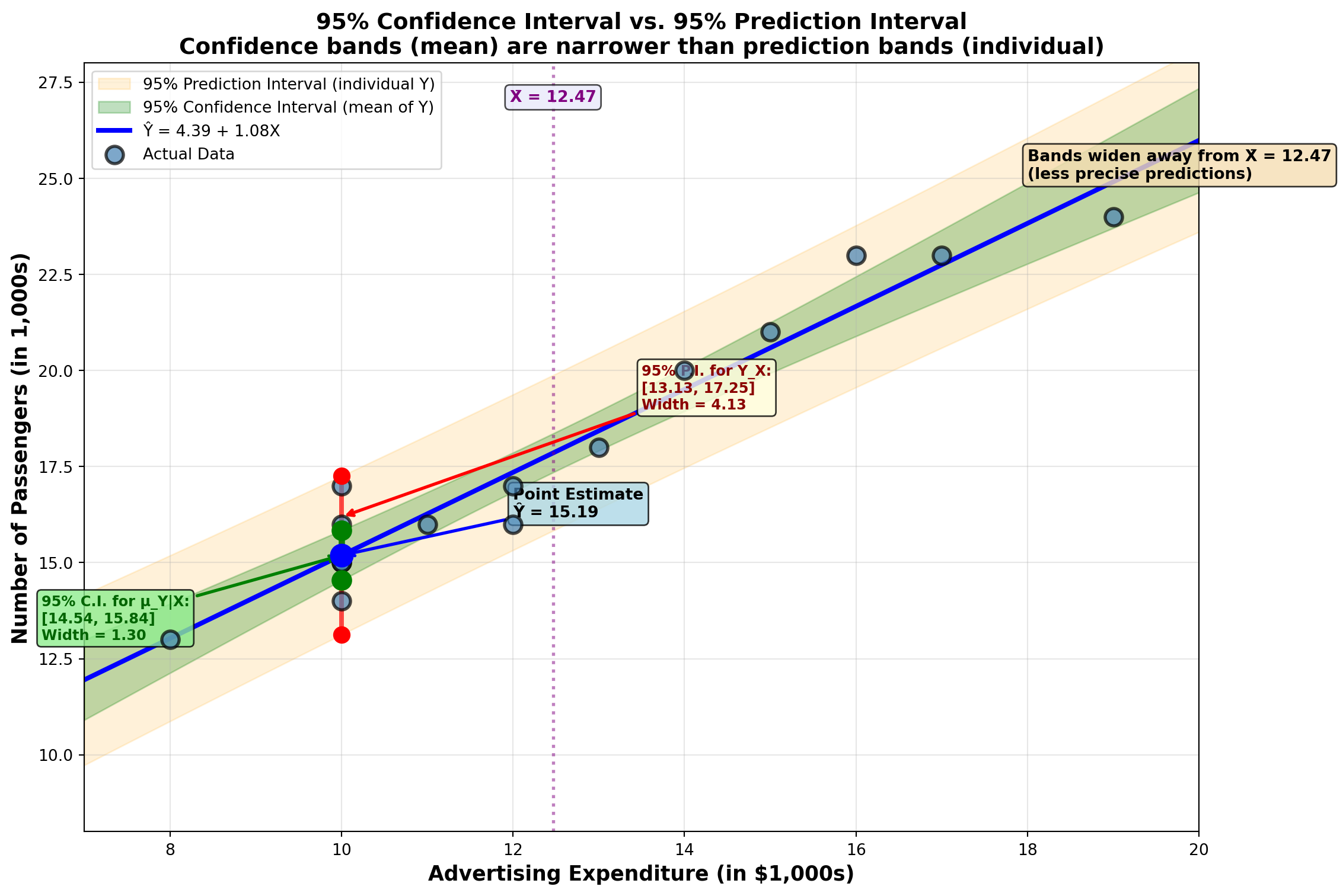
ImportantKey Differences: Confidence vs. Prediction Intervals
| Feature | Confidence Interval | Prediction Interval |
|---|---|---|
| Estimates | Mean of Y (average) | Individual Y (single value) |
| Width | Narrower | Wider |
| Formula | S_{\hat{Y}} = S_e\sqrt{\frac{1}{n} + \frac{(X_i-\bar{X})^2}{SCx}} | S_{Y_X} = S_e\sqrt{1 + \frac{1}{n} + \frac{(X_i-\bar{X})^2}{SCx}} |
| Use Case | “What’s the average outcome?” | “What’s one specific outcome?” |
| Example | Average passengers across many months | Passengers next month |
| Certainty | More certain (means are stable) | Less certain (individuals vary) |
12.21.6 C. Factors Influencing Interval Width
Given a confidence level, we prefer to minimize the interval width. The narrower the interval, the more precise our prediction. Three factors influence width:
- 1. Dispersion of Original Data (S_e)
- More dispersed data → Larger S_e → Wider interval
- 2. Sample Size (n)
- Larger sample → Smaller standard error → Narrower interval
- 3. Distance from Mean (|X_i - \bar{X}|)
- Farther from \bar{X} → Wider interval (regression is based on means, so predictions are less reliable far from the center)
12.22 Section Exercises
Exercise 12.21 (GPA as Predictor of Job Offers) Using the appropriate hypothesis test at the 5% level, is GPA a significant explanatory variable for job offers in Exercise 9? Be sure to show all four hypothesis testing steps.
Exercise 12.22 (Income and Consumption Significance) In Exercise 10, is the relationship between income and consumption significant? Test the hypothesis at a 1% significance level.
Exercise 12.23 (Interest Rate Significance (Two Tests)) In Exercise 11, is the interest rate significant at the 10% level? a. Test the significance of the regression coefficient at 10% b. Test the significance of the correlation coefficient at 10% c. How do these two tests differ?
Exercise 12.24 (Confidence Interval for Average Job Offers) The career placement center at State University (Exercise 9) wants a 95% interval estimate for the average number of job offers that many graduates will receive if they have a GPA of 2.69. Calculate and interpret the appropriate interval.
Exercise 12.25 (Prediction Interval for Fred’s Job Offers) Fred has a GPA of 2.69 (see Exercises 9 and above). Calculate the 95% interval for the number of job offers Fred will receive. Why does this differ from your answer to the previous exercise?
Exercise 12.26 (Confidence Interval for Average Consumption) If the economist at the Florida Department of Human Resources (Exercise 10) identifies many consumers with incomes of $14,200, what is the 99% interval for the average consumption of all those consumers?
Exercise 12.27 (Prediction Interval for Individual Consumer) If the economist from Exercise 10 identifies one consumer with an income of $14,500: a. What is the point estimate of their consumption? b. What is the 99% interval estimate of their consumption?
12.23 Section Summary
TipKey Takeaways: Hypothesis Testing and Intervals
Hypothesis Testing for \beta_1: - Tests whether slope is significantly different from zero
- Uses t = \frac{b_1 - \beta_1}{S_{b_1}} with df = n-2
- If we reject H_0: \beta_1 = 0, the relationship is statistically significant
Hypothesis Testing for \rho: - Tests whether correlation is significantly different from zero
- Uses t = \frac{r - \rho}{S_r} with df = n-2
- In simple regression, gives identical result to testing \beta_1
Confidence Interval for \mu_{Y|X} (Mean): - Estimates average Y when X equals a specific value
- Narrower interval (means are more predictable)
- Formula: \hat{Y}_i \pm t \cdot S_{\hat{Y}}
Prediction Interval for Y_X (Individual): - Estimates a single Y value when X equals a specific value
- Wider interval (individuals more variable)
- Formula: \hat{Y}_i \pm t \cdot S_{Y_X}
For Hop Scotch at X = 10: - Point estimate: 15.19 thousand passengers
- 95% C.I. for mean: [14.54, 15.84]
- 95% P.I. for individual: [13.13, 17.26]
- Both intervals widen as we move away from \bar{X}
12.24 11.12 ANOVA for Regression
The regression model presents a description of the nature of the relationship between dependent and independent variables. We used a t-test to test the hypothesis that \beta_1 = 0. A similar test can be performed using Analysis of Variance (ANOVA) based on the F-test.
The ANOVA procedure measures the amount of variation in the regression model. As noted earlier, there are three sources of variation in a regression model: - Variation explained by regression (SCR) - Unexplained variation due to error (SCE) - Total variation (SCT), which is the sum of the first two
This can be summarized in an ANOVA table.
12.24.1 General ANOVA Table for Regression
Table 11.5: General ANOVA Table
| Source of Variation | Sum of Squares | Degrees of Freedom | Mean Square | F-Ratio |
|---|---|---|---|---|
| Regression | SCR | k | CMR = \frac{SCR}{k} | \frac{CMR}{CME} |
| Error | SCE | n - k - 1 | CME = \frac{SCE}{n-k-1} | |
| Total | SCT | n - 1 |
where k is the number of independent variables (predictors) in the model.
NoteFor Simple Linear Regression
In simple linear regression (one predictor), k = 1, so:
- Regression degrees of freedom: df_R = 1
- Error degrees of freedom: df_E = n - 2
- Total degrees of freedom: df_T = n - 1
12.24.2 Interpreting the F-Ratio
The ratio \frac{CMR}{CME} provides a measure of model accuracy because it compares: - Numerator (CMR): Average squared deviation explained by the model - Denominator (CME): Average squared deviation that remains unexplained
- Higher F-ratio → Better Model
- The model has significant explanatory power.
- Lower F-ratio → Poorer Model
- The model explains little more than random variation.
To determine if the F-ratio is “high enough,” we compare it with a critical value from the F-distribution table.
12.24.3 Computational Formulas
Sum of Squares for Regression
SCR = \frac{(SCxy)^2}{SCx} \quad [11.35]
Sum of Squares for Error (from formula 11.15)
SCE = SCy - \frac{(SCxy)^2}{SCx}
Sum of Squares Total
SCT = SCR + SCE
12.24.4 Application to Hop Scotch Airlines
Using the Hop Scotch data:
Step 1: Calculate SCR
\begin{aligned} SCR &= \frac{(SCxy)^2}{SCx} \\ &= \frac{(148.933333)^2}{137.733333} \\ &= \frac{22,181.14}{137.733333} \\ &= 161.044 \end{aligned}
Step 2: Calculate SCE (already computed earlier)
SCE = 10.689
Step 3: Calculate SCT
SCT = SCR + SCE = 161.044 + 10.689 = 171.733
Step 4: Calculate Mean Squares
CMR = \frac{SCR}{1} = \frac{161.044}{1} = 161.044
CME = \frac{SCE}{13} = \frac{10.689}{13} = 0.822
Step 5: Calculate F-Ratio
F = \frac{CMR}{CME} = \frac{161.044}{0.822} = 195.89
12.24.5 ANOVA Table for Hop Scotch Airlines
Table 11.6: ANOVA Table for Hop Scotch Airlines
| Source of Variation | Sum of Squares | Degrees of Freedom | Mean Square | F-Ratio |
|---|---|---|---|---|
| Regression | 161.04 | 1 | 161.04 | 195.89 |
| Error | 10.69 | 13 | 0.82 | |
| Total | 171.73 | 14 |
12.24.6 Hypothesis Test Using F
Hypotheses:
\begin{aligned} H_0: \beta_1 &= 0 \quad \text{(Model has no explanatory power)} \\ H_A: \beta_1 &\neq 0 \quad \text{(Model is significant)} \end{aligned}
Decision Rule (at \alpha = 0.05):
Critical value: F_{0.05, 1, 13} = 4.67
Do not reject H_0 if F \leq 4.67; otherwise reject H_0.
Conclusion: Since F = 195.89 > 4.67, we reject the null hypothesis. At the 5% significance level, we conclude that advertising has significant explanatory power.
ImportantRelationship Between F-test and t-test
In simple linear regression, the F-test and t-test are mathematically equivalent:
F = t^2
For Hop Scotch: - t = 13.995 - t^2 = (13.995)^2 = 195.86 \approx 195.89 = F
Both tests produce the same conclusion. However, in multiple regression (Chapter 12): - The F-test provides a general test of whether any independent variables have explanatory power - Individual t-tests determine which specific variables are significant
12.25 Solved Problems
12.25.1 Problem 1: Keynes’ Consumption Function
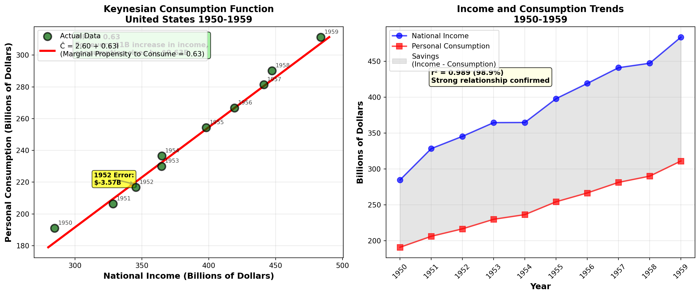
In 1936, British economist John Maynard Keynes published his famous book, The General Theory of Employment, Interest and Money. Keynes proposed a theoretical relationship between income and personal consumption expenditures, arguing that as income increases, consumption increases by a smaller amount.
Milton Friedman, Nobel Prize-winning economist from the University of Chicago, collected data on income and consumption in the United States over an extended period. Here are 10 observations on annual consumption and income levels (in billions of current dollars):
| Year | Income (I) | Consumption (C) |
|---|---|---|
| 1950 | 284.8 | 191.0 |
| 1951 | 328.4 | 206.3 |
| 1952 | 345.5 | 216.7 |
| 1953 | 364.6 | 230.0 |
| 1954 | 364.8 | 236.5 |
| 1955 | 398.0 | 254.4 |
| 1956 | 419.2 | 266.7 |
| 1957 | 441.1 | 281.4 |
| 1958 | 447.3 | 290.1 |
| 1959 | 483.7 | 311.2 |
Required: Derive a consumption function assuming a linear relationship between consumption and income.
12.25.2 Solution
a. Regression Model
Since consumption depends on income, consumption is the dependent variable (Y) and income is the independent variable (X). Friedman sought a consumption function of the form:
\hat{C} = b_0 + b_1 I
Calculations:
\begin{aligned} \sum X &= 3,877.4 \quad \sum Y = 2,484.3 \\ \sum XY &= 984,615.32 \quad \sum X^2 = 1,537,084.88 \quad \sum Y^2 = 630,869.49 \\ n &= 10 \end{aligned}
Sums of Squares and Cross Products:
\begin{aligned} SCx &= \sum X^2 - \frac{(\sum X)^2}{n} \\ &= 1,537,084.88 - \frac{(3,877.4)^2}{10} \\ &= 1,537,084.88 - 1,503,423.076 \\ &= 33,661.804 \end{aligned}
\begin{aligned} SCy &= \sum Y^2 - \frac{(\sum Y)^2}{n} \\ &= 630,869.49 - \frac{(2,484.3)^2}{10} \\ &= 630,869.49 - 617,174.649 \\ &= 13,694.841 \end{aligned}
\begin{aligned} SCxy &= \sum XY - \frac{(\sum X)(\sum Y)}{n} \\ &= 984,615.32 - \frac{(3,877.4)(2,484.3)}{10} \\ &= 984,615.32 - 963,262.482 \\ &= 21,352.838 \end{aligned}
Regression Coefficients:
\begin{aligned} b_1 &= \frac{SCxy}{SCx} \\ &= \frac{21,352.838}{33,661.804} \\ &= 0.634 \end{aligned}
\begin{aligned} b_0 &= \bar{Y} - b_1\bar{X} \\ &= 248.43 - (0.634)(387.74) \\ &= 248.43 - 245.827 \\ &= 2.603 \end{aligned}
Consumption Function:
\hat{C} = 2.603 + 0.63I
Interpretation: - Slope (b_1 = 0.63): For every $1 billion increase in income, consumption increases by $0.63 billion (or 630 million). Economics students will recognize this as the **marginal propensity to consume (MPC)**. - **Intercept (b_0 = 2.603$)**: The consumption level when income is zero (2.603 billion). Economists often argue this interpretation isn’t valid because an economic system always generates positive income.
Example Prediction: For 1952, when I = 345.5:
\hat{C} = 2.603 + 0.63(345.5) = 220.27
Actual consumption was 216.7, resulting in an error of $3.57 billion.
b. Coefficient of Determination
\begin{aligned} r^2 &= \frac{(SCxy)^2}{(SCx)(SCy)} \\ &= \frac{(21,352.838)^2}{(33,661.804)(13,694.841)} \\ &= \frac{455,943,735.1}{461,020,746.4} \\ &= 0.989 \end{aligned}
Interpretation: 98.9% of the variation in consumption is explained by changes in income. This extremely high r^2 confirms Keynes’ theory and demonstrates the strong relationship between income and consumption—vital information for policymakers advising Congress and the President on economic policy.
12.25.3 Problem 2: Federal Reserve Discount Rate Analysis
After approximately six years of continuous expansion, the U.S. economy began showing signs of inflationary pressure in fall 1988. The Federal Reserve attempted to cool inflation by restricting money supply through increasing the discount rate that commercial banks must pay to borrow from the Federal Reserve.
Manuel H. Johnson, Vice Chairman of the Federal Reserve, stated that Fed actions regarding the discount rate could be predicted based on the federal funds rate (the cost banks charge each other for overnight loans). However, Fed watchers argued that the federal funds rate was not serving as an adequate predictor, making it difficult for investors to anticipate interest rate levels.
Data from mid-1987 to mid-1988:
| Date | Federal Funds Rate (%) | Discount Rate (%) |
|---|---|---|
| June 1987 | 8.0 | 7.5 |
| July 1987 | 7.5 | 7.5 |
| Aug 1987 | 7.0 | 7.0 |
| Sept 1987 | 6.5 | 6.5 |
| Oct 1987 | 6.0 | 6.0 |
| Nov 1987 | 6.0 | 5.5 |
| Dec 1987 | 7.0 | 5.5 |
| Jan 1988 | 6.0 | 5.5 |
| Feb 1988 | 7.0 | 5.5 |
| Mar 1988 | 7.5 | 5.5 |
| Apr 1988 | 7.0 | 6.0 |
| May 1988 | 7.5 | 6.5 |
| Totals | 83.0 | 74.5 |
12.25.4 Solution
Since Johnson argued that federal funds rate could explain discount rate behavior, federal funds is the independent variable (X).
a. Regression and Correlation Analysis
Given calculations: \begin{aligned} \sum X &= 83.0 \quad \sum Y = 74.5 \quad n = 12 \\ \sum XY &= 518.5 \quad \sum X^2 = 579 \quad \sum Y^2 = 469.25 \\ \bar{X} &= 6.92 \quad \bar{Y} = 6.21 \end{aligned}
\begin{aligned} SCx &= 4.9167 \quad SCy = 6.7292 \quad SCxy = 3.2083 \\ b_1 &= 0.6525 \quad b_0 = 1.6949 \end{aligned}
Regression Model:
\hat{Y} = 1.69 + 0.653X
Coefficient of Determination:
\begin{aligned} r^2 &= \frac{(SCxy)^2}{(SCx)(SCy)} \\ &= \frac{(3.2083)^2}{(4.92)(6.73)} \\ &= 0.3111 \text{ or } 31.11\% \end{aligned}
r = \sqrt{0.3111} = 0.56
Conclusion: The Fed watchers are correct in their criticism. Only 31% of the changes in the discount rate are explained by changes in the federal funds rate. This is a weak relationship, not suitable for reliable prediction.
b. Standard Error of Estimation
\begin{aligned} SCE &= SCy - \frac{(SCxy)^2}{SCx} \\ &= 6.7292 - \frac{(3.208)^2}{4.9167} \\ &= 4.6303 \end{aligned}
CME = \frac{4.6303}{10} = 0.4630
S_e = \sqrt{0.4630} = 0.6808
Interpretation: Typically, the estimate of the discount rate is in error by 0.68 percentage points—a substantial margin for financial planning.
c. Testing Correlation Significance (95% confidence, df = 10)
\begin{aligned} H_0&: \rho = 0 \\ H_A&: \rho \neq 0 \end{aligned}
Critical value: t_{0.025, 10} = \pm 2.228
\begin{aligned} t &= \frac{r}{S_r} = \frac{r}{\sqrt{(1-r^2)/(n-2)}} \\ &= \frac{0.56}{\sqrt{(1-0.31)/10}} \\ &= \frac{0.56}{0.2627} \\ &= 2.13 \end{aligned}
Decision: Since t = 2.13 < 2.228, we cannot reject H_0. Despite the sample showing a positive relationship, we cannot reject the hypothesis of zero correlation at the 5% significance level.
d. Testing Regression Slope Significance (99% confidence, df = 10)
\begin{aligned} H_0&: \beta_1 = 0 \\ H_A&: \beta_1 \neq 0 \end{aligned}
Critical value: t_{0.005, 10} = \pm 3.169
\begin{aligned} S_{b_1} &= \frac{S_e}{\sqrt{SCx}} = \frac{0.681}{\sqrt{4.92}} = 0.307 \\ t &= \frac{b_1}{S_{b_1}} = \frac{0.6525}{0.307} = 2.126 \end{aligned}
Decision: Since t = 2.126 < 3.169, we cannot reject H_0. The value of b_1 is not significantly different from zero at the 1% level.
Conclusion: There is little to no confidence in the federal funds rate as a predictor of the discount rate. It would be imprudent for investors to rely on federal funds as an indicator of discount rate behavior.
12.26 Formula Summary
NoteEssential Regression Formulas
Basic Regression Line: Y = b_0 + b_1X \quad [11.3]
Sums of Squares: SCx = \sum X^2 - \frac{(\sum X)^2}{n} \quad [11.9] SCy = \sum Y^2 - \frac{(\sum Y)^2}{n} \quad [11.10] SCxy = \sum XY - \frac{(\sum X)(\sum Y)}{n} \quad [11.11]
Regression Coefficients: b_1 = \frac{SCxy}{SCx} \quad [11.12] b_0 = \bar{Y} - b_1\bar{X} \quad [11.13]
Standard Error of Estimation: S_e = \sqrt{\frac{\sum(Y_i - \hat{Y}_i)^2}{n-2}} \quad [11.14] SCE = SCy - \frac{(SCxy)^2}{SCx} \quad [11.15] CME = \frac{SCE}{n-2} \quad [11.16] S_e = \sqrt{CME} \quad [11.17]
Correlation and Determination: r = \frac{SCxy}{\sqrt{(SCx)(SCy)}} \quad [11.23] r^2 = \frac{(SCxy)^2}{(SCx)(SCy)} \quad [11.25]
Hypothesis Tests: t = \frac{b_1 - \beta_1}{S_{b_1}} \quad [11.26] S_{b_1} = \frac{S_e}{\sqrt{SCx}} \quad [11.27] t = \frac{r - \rho}{S_r} \quad [11.29] S_r = \sqrt{\frac{1-r^2}{n-2}} \quad [11.30]
Confidence and Prediction Intervals: S_{\hat{Y}} = S_e\sqrt{\frac{1}{n} + \frac{(X_i - \bar{X})^2}{SCx}} \quad [11.31] \text{C.I. for } \mu_{Y|X} = \hat{Y}_i \pm t \cdot S_{\hat{Y}} \quad [11.32] S_{Y_X} = S_e\sqrt{1 + \frac{1}{n} + \frac{(X_i - \bar{X})^2}{SCx}} \quad [11.33] \text{P.I. for } Y_X = \hat{Y}_i \pm t \cdot S_{Y_X} \quad [11.34]
ANOVA: SCR = \frac{(SCxy)^2}{SCx} \quad [11.35] SCT = SCR + SCE F = \frac{CMR}{CME}
12.27 Chapter Summary
This chapter introduced simple linear regression and correlation analysis, two of the most powerful statistical tools for understanding relationships between variables.
12.27.1 Key Concepts Mastered
1. Regression Analysis - Purpose: Quantify the relationship between dependent (Y) and independent (X) variables - Regression line: \hat{Y} = b_0 + b_1X - Slope (b_1): Change in Y for each one-unit change in X - Intercept (b_0): Value of Y when X = 0 - Method: Ordinary Least Squares (OLS) minimizes \sum(Y_i - \hat{Y}_i)^2
2. Model Evaluation - Standard Error (S_e): Typical prediction error (in units of Y) - Correlation coefficient (r): Strength and direction of linear relationship (-1 \leq r \leq +1) - Coefficient of determination (r^2): Percentage of variation in Y explained by X - ANOVA F-test: Overall significance of the regression model
3. Statistical Inference - Hypothesis tests: Determine if \beta_1 and \rho are significantly different from zero - Confidence intervals: Estimate population parameters (\beta_1, \mu_{Y|X}) - Prediction intervals: Predict individual future values of Y
12.27.2 Critical Distinctions
| Concept | Purpose | Formula | Example (X=10) |
|---|---|---|---|
| Point Estimate | Single prediction | \hat{Y} = b_0 + b_1X | 15.19 |
| Confidence Interval | Estimate mean of Y | Narrower | [14.54, 15.84] |
| Prediction Interval | Estimate individual Y | Wider | [13.13, 17.26] |
12.27.3 Important Cautions
WarningLimitations and Warnings
- Correlation ≠ Causation: High correlation doesn’t prove one variable causes another
- Linear relationships only: r and r^2 only measure linear associations
- Extrapolation danger: Don’t predict beyond the range of observed X values
- Outlier sensitivity: Regression is sensitive to extreme values
- Spurious correlation: Unrelated variables can show correlation by chance
12.27.4 Decision-Making Applications
Regression and correlation analysis enable managers to:
- Forecast: Predict sales, costs, demand based on drivers
- Allocate resources: Optimize spending on advertising, production
- Evaluate performance: Measure relationships between inputs and outputs
- Test theories: Validate economic and business hypotheses with data
- Quantify risk: Understand variability in predictions (via S_e and intervals)
12.27.5 Closing the Cola Wars Scenario
Returning to our opening scenario: Coca-Cola and Pepsi can now use regression to:
- Model sales vs. temperature to optimize production and distribution
- Analyze advertising vs. market share to maximize ROI
- Predict consumption vs. price for pricing strategies
- Forecast seasonal demand patterns for inventory management
With the tools from this chapter, beverage industry managers can make data-driven decisions worth millions of dollars in a $27 billion market.
12.27.6 Looking Ahead
Chapter 12 extends these concepts to multiple regression, where we can use several independent variables simultaneously to predict Y. This provides even more powerful and realistic models for complex business environments.
Congratulations! You’ve mastered simple linear regression and correlation—essential tools that form the foundation for advanced statistical modeling and data science applications in business.
TipChapter 11 Mastery Checklist
You should now be able to: - ✅ Distinguish between dependent and independent variables
- ✅ Create and interpret scatter diagrams
- ✅ Calculate regression coefficients using OLS
- ✅ Interpret slope and intercept in business context
- ✅ Compute and interpret S_e, r, and r^2
- ✅ Test hypotheses about \beta_1 and \rho
- ✅ Construct confidence intervals for means
- ✅ Construct prediction intervals for individuals
- ✅ Perform ANOVA for regression
- ✅ Recognize limitations and avoid common pitfalls