graph TD
    A[The Role of Statistics] --> B[Importance and<br/>necessity of statistics]
    A --> C[Definitions]
    A --> D[Importance<br/>of sampling]
    A --> E[Functions<br/>of statistics]
    A --> F[Opportunities that<br/>statistics offers]
    A --> G[Scales of<br/>measurement]

    C --> C1[Populations<br/>and parameters]
    C --> C2[Samples<br/>and statistics]
    C --> C3[Variables]

    C3 --> C3a[Continuous]
    C3 --> C3b[Discrete]

    D --> D1[Descriptive<br/>statistics]
    D --> D2[Inferential<br/>statistics]
    D --> D3[Sampling error]

    E --> E1[Descriptive<br/>statistics]
    E --> E2[Inferential<br/>statistics]
    E --> E3[Sampling error]

    G --> G1[Nominal]
    G --> G2[Ordinal]
    G --> G3[Interval]
    G --> G4[Ratio]

    style A fill:#e1f5ff,stroke:#333,stroke-width:3px
    style B fill:#c8e6c9,stroke:#333,stroke-width:2px
    style C fill:#fff9c4,stroke:#333,stroke-width:2px
    style D fill:#ffccbc,stroke:#333,stroke-width:2px
    style E fill:#e1bee7,stroke:#333,stroke-width:2px
    style F fill:#b3e5fc,stroke:#333,stroke-width:2px
    style G fill:#f8bbd0,stroke:#333,stroke-width:2px
2 The Role of Statistics
2.1 Business Scenario: Data-Driven Decision Making in the Modern Enterprise
In today’s business environment, organizations face unprecedented complexity and competition. Consider a typical scenario:
Global Manufacturing Corporation operates 47 production facilities across three continents. The Chief Operating Officer needs to answer critical questions:
- Which plants are most productive?
- What factors drive production efficiency?
- How can we predict maintenance needs before equipment fails?
- Are quality standards consistent across all facilities?
- Which regions show the highest employee satisfaction?
Twenty years ago, answering these questions would have required months of manual data collection, calculation, and analysis. Today, statistical methods enable real-time insights from millions of data points.
ImportantThe Statistical Revolution in Business
Statistics has evolved from a specialized academic discipline to an essential business competency.
Organizations that effectively leverage statistical thinking gain competitive advantages:
✓ Faster, better decisions based on evidence rather than intuition
✓ Risk quantification enabling informed trade-offs
✓ Process optimization reducing waste and improving quality
✓ Predictive capabilities anticipating market changes
✓ Performance measurement with objective benchmarks
This chapter introduces the fundamental concepts that make statistical analysis possible and powerful.
2.2 1.1 The Importance and Necessity of Statistics
Statistics permeates modern business and society. From quarterly earnings reports to clinical drug trials, from opinion polls to quality control systems, statistical methods provide the framework for making sense of data and uncertainty.
2.2.1 Why Statistics Matters to Business Professionals
1. Information Overload
Organizations collect vast amounts of data. Statistics provides tools to:
- Summarize large datasets into meaningful insights
- Identify patterns hidden in complexity
- Separate signal from noise
2. Decision Making Under Uncertainty
Business decisions rarely have guaranteed outcomes. Statistics enables:
- Risk assessment and quantification
- Probability-based forecasting
- Confidence intervals for estimates
- Hypothesis testing for strategic choices
3. Competitive Pressure
Companies that master statistical thinking:
- Optimize operations more effectively
- Understand customers more deeply
- Predict market trends more accurately
- Innovate more systematically
4. Regulatory and Quality Requirements
Many industries require statistical evidence:
- Financial reporting and compliance
- Quality control and Six Sigma programs
- Clinical trials for FDA approval
- Environmental impact assessments
2.2.2 Historical Context
The application of statistics to business problems accelerated dramatically in the 20th century:
Early 1900s: Walter Shewhart develops statistical process control at Bell Laboratories
1940s-1950s: W. Edwards Deming brings statistical quality control to Japan
1970s-1980s: Six Sigma methodology emerges
1990s-2000s: Business intelligence and data warehousing expand
2010s-Present: Big data, machine learning, and AI create unprecedented analytical opportunities
NoteStatistics in the Age of AI
While artificial intelligence and machine learning dominate recent headlines, these technologies depend fundamentally on statistical principles:
- Neural networks use statistical optimization
- Model training requires statistical sampling
- Performance evaluation relies on statistical metrics
- Uncertainty quantification uses probabilistic reasoning
Understanding traditional statistics provides the foundation for modern data science and AI.
2.3 1.2 Basic Definitions
To study statistics effectively, we must establish precise definitions for fundamental concepts. These terms form the vocabulary of statistical thinking.
2.3.1 A. Populations and Parameters
In every statistical study, the researcher is interested in a specific collection or set of observations called a population (or universe).
NoteDefinition: Population
Population: The complete collection of all observations of interest to the investigator.
Examples:
- If an economist advising Congress on national tax policy is interested in the incomes of all 165 million wage earners in the United States, then those 165 million incomes constitute the population
- If a tax plan targets earners with incomes above $100,000, then those incomes above $100,000 constitute the population
- If the CEO of a large manufacturing company wants to study production from all company-owned plants, then the production from all these plants is the population
A parameter is any descriptive measure of a population. Examples include:
- The average income of all U.S. wage earners
- The total production of all manufacturing plants
- The proportion of products meeting quality specifications
The key point to remember: A parameter describes a population.
NoteDefinition: Parameter
Parameter: A descriptive measure of the total population of all observations of interest to the investigator.
Important characteristics:
- Usually unknown (populations are too large to measure completely)
- Denoted by Greek letters: \mu (mu) for population mean, \sigma (sigma) for population standard deviation, \pi or p for population proportion
- Fixed values (don’t change with sampling)
- The target of statistical inference
2.3.2 B. Samples and Statistics
Although statisticians are generally interested in some aspect of an entire population, they frequently discover that populations are too large to study in their entirety. Calculating the average income of each of the 165 million wage earners would be an overwhelming task.
Consequently, it is usually sufficient to study only a small portion of the population. This smaller, more manageable portion is called a sample. A sample is a subset of the population selected scientifically.
NoteDefinition: Sample
Sample: A representative part of the population selected for study because the population is too large to analyze in its entirety.
Examples:
- Each month, the U.S. Department of Labor calculates the average income of a sample of several thousand wage earners selected from the total population of 165 million workers
- A quality inspector examines 50 bottles from a production run of 10,000
- A political pollster surveys 1,200 voters from an electorate of 80 million
Why are samples necessary? Studying complete populations is:
- Too expensive
- Too time-consuming
- Sometimes impossible (destructive testing)
- Often unnecessary (well-designed samples provide reliable information)
A statistic is a descriptive measure of a sample. The average income of those several thousand workers calculated by the Department of Labor is a statistic. The statistic is to the sample what the parameter is to the population.
The statistic serves as an estimate of the parameter. Although we’re really interested in the value of the population parameter, we often must be content with calculating it using a sample statistic.
NoteDefinition: Statistic
Statistic: A value that describes a sample and serves as an estimate of the corresponding population parameter.
Important characteristics:
- Calculated from sample data (known values)
- Denoted by Roman letters: \bar{x} (x-bar) for sample mean, s for sample standard deviation, \hat{p} for sample proportion
- Variable (changes from sample to sample)
- Used to estimate unknown population parameters
Table 1.1: Population Parameters vs. Sample Statistics
| Measure | Population (Parameter) | Sample (Statistic) |
|---|---|---|
| Mean | \mu (mu) | \bar{x} (x-bar) |
| Standard Deviation | \sigma (sigma) | s |
| Proportion | \pi or p | \hat{p} (p-hat) |
| Size | N | n |
| Variance | \sigma^2 | s^2 |
2.3.3 C. Variables
A variable is the characteristic of the sample or population being observed. If the mayor of San Francisco’s statistical advisor is interested in the distance that daily commuters travel to work each morning, the variable is miles traveled. In a study of U.S. wage earners’ income, the variable is income.
NoteDefinition: Variable
Variable: A characteristic of the population being analyzed in a statistical study.
Variables can be classified in two important ways:
1. Quantitative vs. Qualitative Variables
Quantitative variables can be expressed numerically:
- Income of wage earners
- Height of individuals
- Test scores
- Miles traveled to work
- Sales revenue
- Production output
Qualitative variables are measured non-numerically:
- Marital status of credit applicants (single, married, divorced, widowed)
- Gender of students (male, female, non-binary)
- Race, hair color, religious preference
- Product quality classification (acceptable, defective)
- Customer satisfaction level (very satisfied, satisfied, neutral, dissatisfied)
2. Continuous vs. Discrete Variables
Continuous variables can take any value within a given range. No matter how close two observations are, if the measuring instrument is precise enough, a third observation can be found between them. Continuous variables generally result from measurement.
Examples:
- Temperature (70.1°F, 70.15°F, 70.153°F…)
- Time (3.5 seconds, 3.52 seconds, 3.518 seconds…)
- Weight, height, distance, pressure
Discrete variables are limited to certain values, usually integers. They often result from counting or enumeration.
Examples:
- Number of students in a class (0, 1, 2, 3… never 2.5 students)
- Number of cars sold by General Motors
- Number of defective products in a batch
- Number of customers served
TipPractical Distinction: Measurement vs. Counting
Quick rule:
- If you measure it (ruler, scale, thermometer, clock) → Usually continuous
- If you count it (1, 2, 3…) → Usually discrete
Some variables that are technically discrete (like age in years) are often treated as continuous when the number of possible values is large.
Throughout the study of statistics, we will refer repeatedly to these concepts and terms. You should be aware of the role each plays in the statistical analysis process. It is especially important to be able to differentiate between:
- A population and its parameters
- A sample and its statistics
2.4 1.3 The Importance of Sampling
Much of a statistician’s work is done with samples. Samples are necessary because populations are often too large to study in their entirety. It is very costly and time-consuming to examine the entire population, so a sample must be selected from the population, the sample statistic calculated, and used to estimate the corresponding population parameter.
This analysis of samples involves a distinction between the two main branches of statistical analysis:
2.4.1 A. Descriptive Statistics
Descriptive statistics is the process of collecting, grouping, and presenting data in a manner that describes the data easily and quickly.
Purpose:
- Summarize large datasets
- Create visual representations (charts, graphs)
- Calculate summary measures (averages, percentages)
- Organize data for easy interpretation
Examples:
- A company’s quarterly earnings report
- A histogram showing employee salary distribution
- Average customer satisfaction score
- Percentage of defective products
NoteDefinition: Descriptive Statistics
Descriptive Statistics: Methods for organizing, summarizing, and presenting data in an informative way.
Chapters 2 and 3 examine descriptive statistics and illustrate the various methods and tools that can be used to present and summarize large datasets.
2.4.2 B. Inferential Statistics
Inferential statistics involves using a sample to draw some inference or conclusion about the population from which the sample is part.
Purpose:
- Estimate population parameters from sample statistics
- Test hypotheses about populations
- Make predictions
- Quantify uncertainty
Examples:
- Using a sample of 2,000 voters to predict election results
- Testing whether a new drug is effective based on clinical trial data
- Estimating average lifetime of lightbulbs from a sample
- Determining if a production process meets quality standards
NoteDefinition: Inferential Statistics
Inferential Statistics: Methods for using sample data to make generalizations, estimates, predictions, or decisions about a larger population.
When the U.S. Department of Labor uses the average income of a sample of several thousand workers to estimate the average income of 165 million workers, it is using a simple form of inferential statistics.
The Relationship Between Descriptive and Inferential Statistics:
Code
import matplotlib.pyplot as plt
import matplotlib.patches as mpatches
from matplotlib.patches import FancyBboxPatch, FancyArrowPatch

fig, ax = plt.subplots(figsize=(14, 8))
ax.set_xlim(0, 10)
ax.set_ylim(0, 10)
ax.axis('off')

# Population box
pop_box = FancyBboxPatch((0.5, 6), 2.5, 2.5, boxstyle="round,pad=0.1",
                         edgecolor='darkblue', facecolor='lightblue', linewidth=3)
ax.add_patch(pop_box)
ax.text(1.75, 7.75, 'POPULATION', ha='center', va='center', fontsize=14, fontweight='bold')
ax.text(1.75, 7.3, 'N = 165 million', ha='center', va='center', fontsize=10)
ax.text(1.75, 6.9, 'Parameter: μ', ha='center', va='center', fontsize=11, style='italic')
ax.text(1.75, 6.5, '(Unknown)', ha='center', va='center', fontsize=9, color='red')

# Sampling arrow
arrow1 = FancyArrowPatch((3, 7.25), (4.5, 7.25), arrowstyle='->',
                         mutation_scale=30, linewidth=2.5, color='darkgreen')
ax.add_patch(arrow1)
ax.text(3.75, 7.6, 'Sampling', ha='center', fontsize=11, fontweight='bold', color='darkgreen')

# Sample box
sample_box = FancyBboxPatch((4.5, 6), 2.5, 2.5, boxstyle="round,pad=0.1",
                           edgecolor='darkgreen', facecolor='lightgreen', linewidth=3)
ax.add_patch(sample_box)
ax.text(5.75, 7.75, 'SAMPLE', ha='center', va='center', fontsize=14, fontweight='bold')
ax.text(5.75, 7.3, 'n = 2,000', ha='center', va='center', fontsize=10)
ax.text(5.75, 6.9, 'Statistic: x̄', ha='center', va='center', fontsize=11, style='italic')
ax.text(5.75, 6.5, '(Calculated)', ha='center', va='center', fontsize=9, color='green')

# Descriptive statistics arrow
arrow2 = FancyArrowPatch((5.75, 6), (5.75, 4.5), arrowstyle='->',
                         mutation_scale=30, linewidth=2.5, color='purple')
ax.add_patch(arrow2)
ax.text(6.5, 5.25, 'Descriptive\nStatistics', ha='center', fontsize=10,
        fontweight='bold', color='purple')

# Descriptive box
desc_box = FancyBboxPatch((4.5, 2.5), 2.5, 1.8, boxstyle="round,pad=0.1",
                         edgecolor='purple', facecolor='plum', linewidth=2)
ax.add_patch(desc_box)
ax.text(5.75, 3.9, 'Organize & Summarize', ha='center', fontsize=11, fontweight='bold')
ax.text(5.75, 3.5, '• Charts/Graphs', ha='center', fontsize=9)
ax.text(5.75, 3.2, '• Tables', ha='center', fontsize=9)
ax.text(5.75, 2.9, '• Summary Measures', ha='center', fontsize=9)

# Inference arrow
arrow3 = FancyArrowPatch((4.5, 7.25), (3, 7.25), arrowstyle='->',
                         mutation_scale=30, linewidth=2.5, color='darkorange')
ax.add_patch(arrow3)
ax.text(3.75, 6.9, 'Inference', ha='center', fontsize=11, fontweight='bold', color='darkorange')

# Inferential statistics box
inf_box = FancyBboxPatch((0.5, 2.5), 2.5, 1.8, boxstyle="round,pad=0.1",
                        edgecolor='darkorange', facecolor='lightyellow', linewidth=2)
ax.add_patch(inf_box)
ax.text(1.75, 3.9, 'Make Inferences', ha='center', fontsize=11, fontweight='bold')
ax.text(1.75, 3.5, '• Estimate μ using x̄', ha='center', fontsize=9)
ax.text(1.75, 3.2, '• Test Hypotheses', ha='center', fontsize=9)
ax.text(1.75, 2.9, '• Predict', ha='center', fontsize=9)

# Inference connection
arrow4 = FancyArrowPatch((1.75, 6), (1.75, 4.5), arrowstyle='->',
                         mutation_scale=30, linewidth=2.5, color='darkorange', linestyle='--')
ax.add_patch(arrow4)
ax.text(0.8, 5.25, 'Inferential\nStatistics', ha='center', fontsize=10,
        fontweight='bold', color='darkorange')

# Title
ax.text(5, 9.3, 'The Statistical Process: From Population to Inference',
        ha='center', fontsize=15, fontweight='bold')

# Note about uncertainty
uncertainty_box = FancyBboxPatch((3.5, 0.8), 3, 1, boxstyle="round,pad=0.1",
                                edgecolor='red', facecolor='mistyrose', linewidth=2)
ax.add_patch(uncertainty_box)
ax.text(5, 1.5, '⚠️  Sampling Error Possible', ha='center', fontsize=11,
        fontweight='bold', color='darkred')
ax.text(5, 1.1, 'x̄ may not exactly equal μ', ha='center', fontsize=9, style='italic')

plt.tight_layout()
plt.show()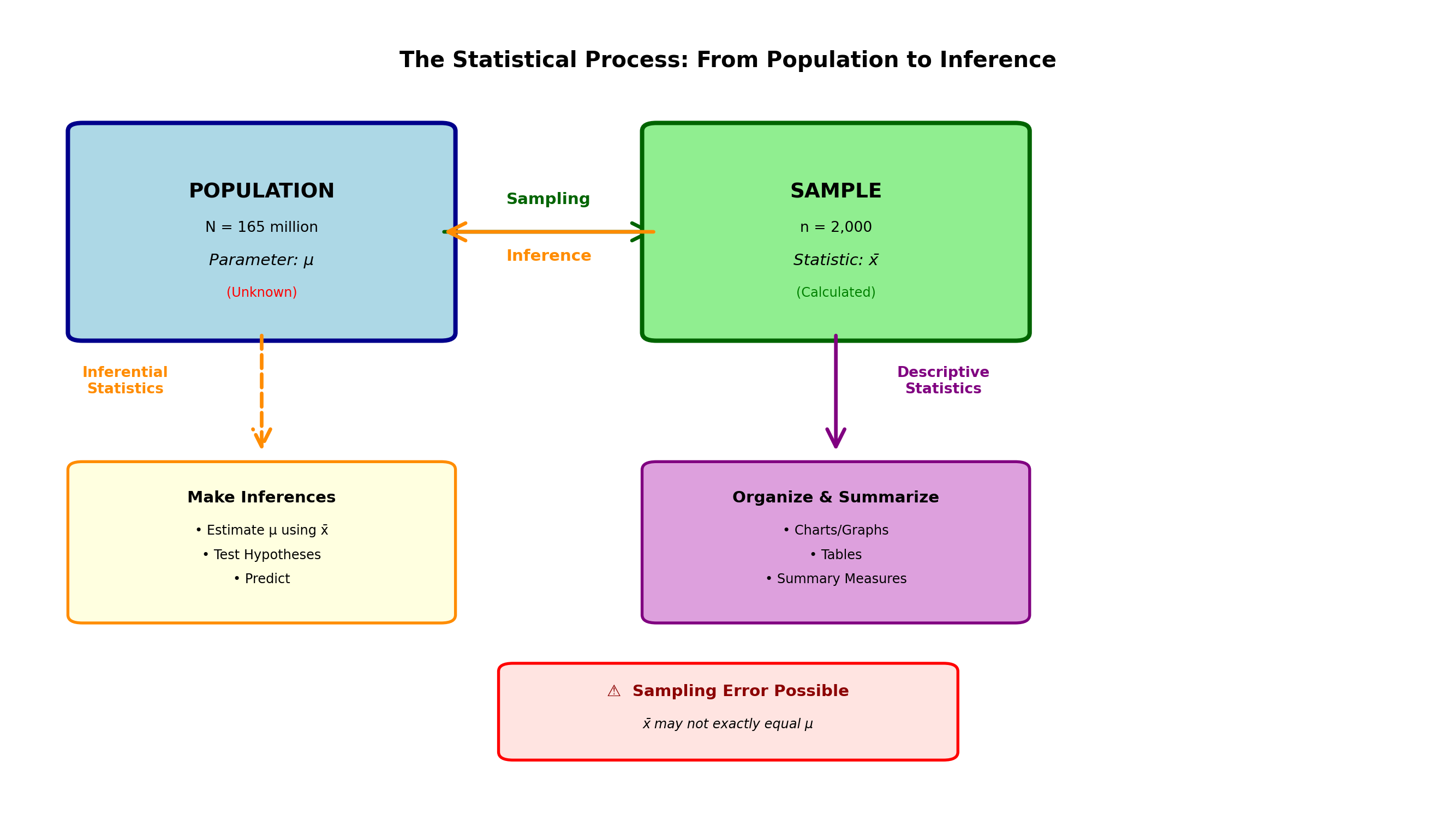
2.4.3 C. Sampling Error
The accuracy of any estimate is of enormous importance. This accuracy depends largely on how the sample was taken and the care taken to ensure that the sample provides a reliable picture of the population.
However, very frequently it is found that the sample is not entirely representative of the population, resulting in sampling error.
NoteDefinition: Sampling Error
Sampling Error: The difference between the unknown population parameter and the sample statistic used to estimate the parameter.
\text{Sampling Error} = \text{Statistic} - \text{Parameter}
For example: \text{Error} = \bar{x} - \mu (sample mean minus population mean)
Two Possible Causes of Sampling Error:
1. Random Chance in the Sampling Process
Due to the chance factor in selecting sample elements, it’s possible to unknowingly select atypical elements that don’t represent the population.
Example:
In attempting to estimate the population mean, you might select sample elements that are abnormally large, producing an overestimation of the population mean. Conversely, chance might produce many unusually small sample elements, causing an underestimation. In either case, sampling error has occurred.
2. Sample Bias
Sample bias is a more serious form of sampling error. Bias occurs when there is some tendency to select certain sample elements instead of others.
WarningDefinition: Sample Bias
Sample Bias: The tendency to favor the selection of certain sample elements over others.
If the sampling process is designed incorrectly and tends to promote the selection of too many units with a particular characteristic at the expense of units without that characteristic, the sample is said to be biased.
Examples of bias:
- A process that inherently favors selecting men while excluding women
- Surveys conducted only during business hours (excluding working people)
- Online polls (excluding those without internet access)
- Voluntary response surveys (only highly motivated people respond)
A more rigorous treatment of sampling bias will be presented in a later chapter. Although sampling error can never be measured (because the parameter remains unknown), you should be aware that the probability of its occurrence exists.
ImportantManaging Sampling Error
Cannot be eliminated, but can be controlled:
✓ Larger sample sizes reduce random sampling error
✓ Proper sampling design eliminates bias
✓ Random selection ensures representativeness
✓ Statistical inference quantifies uncertainty
Later chapters will teach techniques for:
- Calculating confidence intervals (quantifying uncertainty)
- Determining appropriate sample sizes
- Testing hypotheses with known error probabilities
2.5 1.4 The Functions of Statistics
Repeatedly we have emphasized the usefulness of statistics and the wide variety of problems it can solve. To more fully illustrate this broad applicability, it’s necessary to examine the various functions of statistics.
Statistics is the science concerned with:
1. Collection of data
2. Organization of data
3. Presentation of data
4. Analysis of data
5. Interpretation of data
Although in every statistical study the first step is data collection, it is usual in a basic statistics course to assume that data have already been collected and are now available. Therefore, work begins with the effort to organize and present these data in a meaningful and descriptive manner.
2.5.1 The Statistical Process
Code
import matplotlib.pyplot as plt
import matplotlib.patches as mpatches
from matplotlib.patches import FancyBboxPatch, FancyArrowPatch, Circle

fig, ax = plt.subplots(figsize=(14, 10))
ax.set_xlim(0, 10)
ax.set_ylim(0, 10)
ax.axis('off')

# Define positions for circular flow
positions = [
    (5, 8.5),    # 1. Collection
    (7.5, 6.5),  # 2. Organization
    (7.5, 3.5),  # 3. Presentation
    (5, 1.5),    # 4. Analysis
    (2.5, 3.5),  # 5. Interpretation
    (2.5, 6.5),  # Back to Collection
]

colors = ['#FFB6C1', '#FFD700', '#90EE90', '#87CEEB', '#DDA0DD']
labels = [
    '1. COLLECTION',
    '2. ORGANIZATION',
    '3. PRESENTATION',
    '4. ANALYSIS',
    '5. INTERPRETATION'
]

descriptions = [
    'Gather relevant data\n• Surveys\n• Experiments\n• Databases',
    'Structure the data\n• Sort\n• Group\n• Categorize',
    'Display findings\n• Tables\n• Charts\n• Graphs',
    'Calculate measures\n• Means\n• Correlations\n• Tests',
    'Draw conclusions\n• Decisions\n• Predictions\n• Recommendations'
]

# Draw circles and text
for i in range(5):
    x, y = positions[i]

    # Circle
    circle = Circle((x, y), 0.7, facecolor=colors[i], edgecolor='darkblue', linewidth=3)
    ax.add_patch(circle)

    # Number
    ax.text(x, y + 0.15, str(i + 1), ha='center', va='center',
            fontsize=24, fontweight='bold', color='darkblue')

    # Label
    ax.text(x, y - 0.25, labels[i].split('. ')[1], ha='center', va='center',
            fontsize=11, fontweight='bold')

    # Description box
    if i == 0:  # Top
        desc_x, desc_y = x, y + 1.2
    elif i == 1:  # Right upper
        desc_x, desc_y = x + 1.5, y
    elif i == 2:  # Right lower
        desc_x, desc_y = x + 1.5, y
    elif i == 3:  # Bottom
        desc_x, desc_y = x, y - 1.2
    else:  # Left
        desc_x, desc_y = x - 1.5, y

    desc_box = FancyBboxPatch((desc_x - 0.9, desc_y - 0.45), 1.8, 0.9,
                              boxstyle="round,pad=0.05", edgecolor=colors[i],
                              facecolor='white', linewidth=1.5, alpha=0.9)
    ax.add_patch(desc_box)

    # Multi-line description
    lines = descriptions[i].split('\n')
    y_offset = desc_y + 0.25
    for line in lines:
        ax.text(desc_x, y_offset, line, ha='center', va='center', fontsize=8)
        y_offset -= 0.2

# Draw arrows connecting the circles
for i in range(5):
    x1, y1 = positions[i]
    x2, y2 = positions[(i + 1) % 6]

    if i < 4:
        # Calculate arrow positions to start/end at circle edge
        angle = plt.np.arctan2(y2 - y1, x2 - x1)
        x1_edge = x1 + 0.7 * plt.np.cos(angle)
        y1_edge = y1 + 0.7 * plt.np.sin(angle)
        x2_edge = x2 - 0.7 * plt.np.cos(angle)
        y2_edge = y2 - 0.7 * plt.np.sin(angle)

        arrow = FancyArrowPatch((x1_edge, y1_edge), (x2_edge, y2_edge),
                               arrowstyle='->', mutation_scale=25, linewidth=3,
                               color='darkblue', alpha=0.6)
        ax.add_patch(arrow)

# Cycle arrow from 5 back to 1
arrow_cycle = FancyArrowPatch((2.5, 7.2), (2.5, 7.8),
                             arrowstyle='->', mutation_scale=25, linewidth=2,
                             color='darkgreen', linestyle='--', alpha=0.7)
ax.add_patch(arrow_cycle)
ax.text(1.5, 7.5, 'Continuous\nImprovement\nCycle', ha='center', fontsize=9,
        color='darkgreen', fontweight='bold', style='italic')

# Title
ax.text(5, 9.6, 'The Statistical Process: A Continuous Cycle',
        ha='center', fontsize=16, fontweight='bold')

# Central concept
center_box = FancyBboxPatch((4, 4.5), 2, 1, boxstyle="round,pad=0.1",
                           edgecolor='darkred', facecolor='lightyellow', linewidth=2.5)
ax.add_patch(center_box)
ax.text(5, 5.3, 'Data-Driven', ha='center', fontsize=13, fontweight='bold', color='darkred')
ax.text(5, 4.8, 'Decision Making', ha='center', fontsize=13, fontweight='bold', color='darkred')

plt.tight_layout()
plt.show()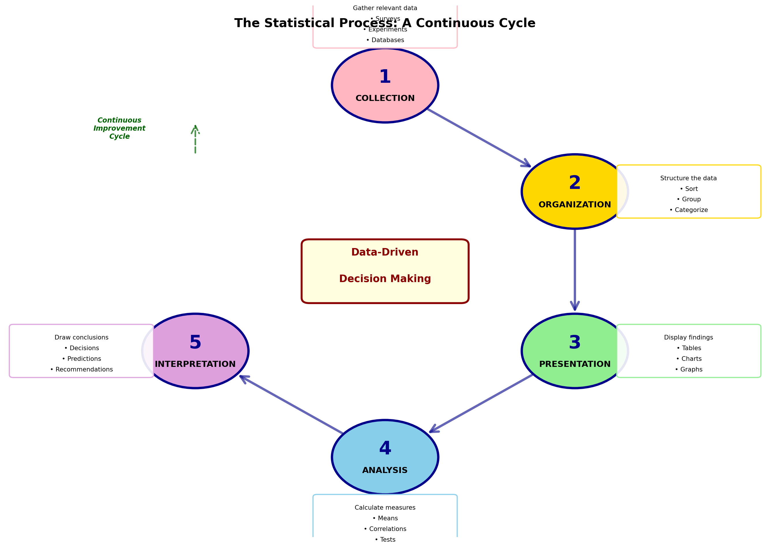
Data must be placed in a logical order that quickly and easily reveals the message they contain. This procedure constitutes the process of descriptive statistics, as defined and discussed in the following chapters.
After data have been organized and presented for review, the statistician must analyze and interpret them. These procedures are based on inferential statistics and constitute an important benefit of statistical analysis by helping in the decision-making and problem-solving process.
2.5.2 Prediction and Forecasting
You will discover that through the application of precise statistical procedures, it is possible to predict the future with a certain degree of accuracy.
Any business facing competitive pressures can benefit considerably from the ability to anticipate business conditions before they occur. If a company knows what its sales will be at some point in the near future, management can make more accurate and effective plans regarding current operations.
If future sales are estimated with a reliable degree of accuracy, management can easily make important decisions regarding:
- Inventory levels
- Raw material orders
- Employee hiring
- Virtually every aspect of business operations
TipBusiness Applications of Statistical Functions
Manufacturing:
- Quality control charts (collection, analysis)
- Process optimization (organization, interpretation)
- Defect prediction (analysis, interpretation)
Marketing:
- Customer surveys (collection)
- Market segmentation (organization)
- Sales dashboards (presentation)
- Campaign effectiveness (analysis)
- Strategic recommendations (interpretation)
Finance:
- Transaction data (collection)
- Risk categorization (organization)
- Portfolio reports (presentation)
- Performance metrics (analysis)
- Investment decisions (interpretation)
Human Resources:
- Employee data (collection)
- Compensation bands (organization)
- Diversity dashboards (presentation)
- Turnover analysis (analysis)
- Retention strategies (interpretation)
2.6 1.5 Opportunities That Statistics Offers
The study and application of statistics opens numerous professional and business opportunities. Organizations across all industries seek individuals who can work effectively with data.
2.6.1 Career Opportunities
Data Analyst
- Examine data to identify trends and patterns
- Create visualizations and reports
- Support business decision-making
Business Intelligence Analyst
- Design dashboards and reporting systems
- Analyze KPIs (Key Performance Indicators)
- Provide actionable insights
Market Research Analyst
- Design and analyze surveys
- Study consumer behavior
- Forecast market trends
Operations Analyst
- Optimize processes and workflows
- Apply statistical process control
- Improve efficiency and quality
Financial Analyst
- Analyze investment performance
- Model risk and return
- Support portfolio management
Data Scientist (advanced)
- Build predictive models
- Apply machine learning
- Extract insights from big data
2.6.2 Competitive Advantages for Organizations
Companies that effectively leverage statistical thinking gain advantages in:
1. Quality and Efficiency
- Six Sigma programs reduce defects
- Statistical process control maintains consistency
- Design of experiments optimizes products and processes
2. Customer Understanding
- Segmentation analysis identifies target markets
- Satisfaction surveys measure performance
- Predictive models anticipate needs
3. Risk Management
- Credit scoring models assess default probability
- Portfolio theory optimizes risk/return trade-offs
- Stress testing evaluates resilience
4. Strategic Planning
- Forecasting methods predict demand
- Scenario analysis evaluates alternatives
- A/B testing validates decisions
ImportantThe Statistical Mindset
Beyond specific techniques, statistics cultivates a way of thinking:
✓ Evidence-based reasoning: Decisions supported by data, not just intuition
✓ Quantification of uncertainty: Explicit acknowledgment of what we don’t know
✓ Critical evaluation: Questioning assumptions and examining claims
✓ Systematic approach: Structured methods for problem-solving
✓ Continuous learning: Using feedback to improve over time
This mindset is valuable in any career and essential in data-driven roles.
2.7 1.6 Scales of Measurement
Variables can be classified based on their scale of measurement. The way variables are classified greatly affects how they are used in analysis. Variables can be:
- Nominal
- Ordinal
- Interval
- Ratio
Understanding these scales is crucial because they determine:
- Which statistical methods are appropriate
- What mathematical operations make sense
- How to interpret results correctly
2.7.1 A. Nominal Scale
A nominal measurement is created when names are used to establish categories within which variables can be recorded exclusively.
NoteDefinition: Nominal Scale
Nominal Scale: Names or classifications used for data in distinct and separate categories.
Characteristics:
- Categories are mutually exclusive
- No inherent order or ranking
- Numbers (if used) are merely labels
- Mathematical operations are meaningless
Examples:
Gender: Male, Female, Non-binary
- Could be coded as 1, 2, 3, but these numbers only indicate categories
- Cannot meaningfully calculate “average gender”
Soft Drinks: Coca-Cola, Pepsi, 7-Up, Dr Pepper
- Each beverage can be recorded in one category, excluding others
Department: Sales, Marketing, Finance, Operations, HR
- Categories have no inherent ordering
Table 1.2: Investment Fund Classifications (Nominal Scale)
| Category | Fund Name |
|---|---|
| Aggressive Growth | Twenty Century Growth |
| Janus | |
| Total Return | Scudder |
| Vanguard Star | |
| Pax World | |
| USAA Cornerstone | |
| Bonds | Strong Short-Term |
| Scudder Short-Term | |
| Money Market Funds | Alger Portfolio |
| Mariner Government | |
| Tax-Exempt | Kemper Municipals |
Important to remember: A nominal scale measurement indicates no order of preference, but simply establishes a categorical arrangement in which each observation can be placed.
Appropriate statistics for nominal data:
- Frequency counts
- Mode (most common category)
- Proportions and percentages
- Chi-square tests
2.7.2 B. Ordinal Scale
Unlike a nominal scale measurement, an ordinal scale measurement does show an ordering or sequencing of the data. Observations are ranked based on some criteria.
NoteDefinition: Ordinal Scale
Ordinal Scale: Measurements that classify observations in categories with a meaningful order.
Characteristics:
- Categories can be ranked or ordered
- Differences between ranks are not necessarily equal
- Numbers indicate relative position
- Only ranking matters, not magnitude
Examples:
Sears Product Ratings: Good, Better, Best
- Clear ordering exists
- “Best” is preferred to “Good”
- But “Better” is not necessarily twice as good as “Good”
Opinion Survey Responses:
- Strongly Agree
- Agree
- No Opinion
- Disagree
- Strongly Disagree
Education Level:
- High School
- Bachelor’s Degree
- Master’s Degree
- Doctoral Degree
Just as with nominal data, numbers can be used to order the ranks. Sears could have used ranks of “1”, “2”, and “3”, or “1”, “3”, and “12” for that matter. The arithmetic differences between the values are meaningless. A product with rank “2” is not necessarily two times better than one with rank “1”.
Table 1.3: Ordinal Ranking of Investment Risk
| Investment | Risk Factor |
|---|---|
| Gold | Very High |
| Small Growth Companies | Very High |
| Maximum Capital Gain | High |
| International | High |
| Option Income | Low |
| Balanced | Low |
Note that the ranks of “Very High”, “High”, and “Low” could have been based on values “1”, “2”, and “3”, or “A”, “B”, and “C”. But the actual differences in risk levels cannot be meaningfully measured. We only know that a “High” risk investment has greater risk than a “Low” risk investment.
Appropriate statistics for ordinal data:
- Median (middle rank)
- Percentiles
- Spearman rank correlation
- Non-parametric tests (Mann-Whitney, Kruskal-Wallis)
2.7.3 C. Interval Scale
On an interval scale, variables are measured numerically, and like ordinal data, carry an inherent rank or ordering. However, unlike ordinal ranks, the difference between values is important.
NoteDefinition: Interval Scale
Interval Scale: Measurements on a numerical scale in which the value of zero is arbitrary but the difference between values is meaningful.
Characteristics:
- Numerical measurements
- Equal intervals have equal meaning
- Zero point is arbitrary (not absolute zero)
- Ratios are not meaningful
Examples:
Temperature (Fahrenheit or Celsius):
- 70°F is not just higher than 60°F
- The same difference of 10 degrees exists between 90°F and 100°F
- BUT: Zero is arbitrary
- 80°F is not twice as hot as 40°F (ratio is meaningless)
Calendar Years:
- Year 2020, 2021, 2022
- Equal intervals (years) have equal meaning
- But “Year 0” is an arbitrary starting point
IQ Scores:
- Difference between IQ 100 and 110 equals difference between 110 and 120
- But IQ 150 is not “1.5 times as intelligent” as IQ 100
On an interval scale, the value of zero is selected arbitrarily. There is nothing concrete that forced setting zero degrees; it is simply an arbitrary reference point. The Fahrenheit scale could have been created so that zero was set at a warmer (or colder) temperature.
Zero is not given a special meaning other than being 10 degrees colder than 10°F. Thus, 80 degrees is not twice as hot as 40 degrees, and the ratio 80/40 has no meaning.
Appropriate statistics for interval data:
- Mean, median, mode
- Standard deviation
- Correlation
- t-tests, ANOVA
- Regression analysis
2.7.4 D. Ratio Scale
The ratio scale is the highest level of measurement. It has all the properties of an interval scale, plus a meaningful absolute zero point.
NoteDefinition: Ratio Scale
Ratio Scale: The highest level of measurement in which both differences and ratios are meaningful, and there exists a true zero point.
Characteristics:
- All properties of interval scale
- True zero point (absolute absence)
- Ratios are meaningful
- All mathematical operations valid
Examples:
Weight:
- 0 pounds means complete absence of weight
- 60 pounds is twice as heavy as 30 pounds
- Ratio 60/30 = 2 is meaningful
Income:
- $0 income means no income at all
- $100,000 is twice $50,000
- All arithmetic operations valid
Sales Revenue:
- Zero sales = no revenue
- $2 million is double $1 million
Number of Employees:
- Zero employees = no employees
- 100 employees is 10 times 10 employees
Time Duration:
- 0 seconds = no time elapsed
- 10 seconds is twice as long as 5 seconds
With ratio scales, statements like “twice as much” or “three times greater” have real meaning.
Appropriate statistics for ratio data:
- All statistics applicable to interval data
- Plus: Geometric mean, coefficient of variation
- Meaningful percentage changes
- Ratios and proportions
2.7.5 Comparing the Four Scales
Table 1.4: Summary of Measurement Scales
| Scale | Order | Equal Intervals | True Zero | Examples | Appropriate Statistics |
|---|---|---|---|---|---|
| Nominal | No | No | No | Gender, Color, Product Category | Frequency, Mode, Chi-square |
| Ordinal | Yes | No | No | Rankings, Satisfaction Levels | Median, Percentiles, Non-parametric tests |
| Interval | Yes | Yes | No | Temperature (°F/°C), IQ, Years | Mean, SD, Correlation, t-tests, ANOVA |
| Ratio | Yes | Yes | Yes | Weight, Income, Sales, Age, Count | All statistics including Geometric Mean |
Code
import matplotlib.pyplot as plt
import matplotlib.patches as mpatches
from matplotlib.patches import FancyBboxPatch, Rectangle

fig, ax = plt.subplots(figsize=(14, 10))
ax.set_xlim(0, 10)
ax.set_ylim(0, 10)
ax.axis('off')

# Title
ax.text(5, 9.5, 'Hierarchy of Measurement Scales',
        ha='center', fontsize=16, fontweight='bold')

# Pyramid levels
levels = [
    {'y': 1, 'height': 1.5, 'width': 8, 'color': '#FF6B6B', 'name': 'NOMINAL',
     'properties': 'Categories Only', 'example': 'Gender: Male, Female'},
    {'y': 2.7, 'height': 1.5, 'width': 6.5, 'color': '#FFA500', 'name': 'ORDINAL',
     'properties': '+ Ranking', 'example': 'Good, Better, Best'},
    {'y': 4.4, 'height': 1.5, 'width': 5, 'color': '#FFD700', 'name': 'INTERVAL',
     'properties': '+ Equal Intervals', 'example': 'Temperature: 70°F, 80°F'},
    {'y': 6.1, 'height': 1.5, 'width': 3.5, 'color': '#90EE90', 'name': 'RATIO',
     'properties': '+ True Zero', 'example': 'Income: $50,000, $100,000'}
]

for i, level in enumerate(levels):
    # Trapezoid shape for pyramid
    x_center = 5
    half_width = level['width'] / 2

    # Draw the box
    box = FancyBboxPatch((x_center - half_width, level['y']), level['width'], level['height'],
                         boxstyle="round,pad=0.05", edgecolor='darkblue',
                         facecolor=level['color'], linewidth=3, alpha=0.8)
    ax.add_patch(box)

    # Scale name
    ax.text(x_center, level['y'] + level['height'] - 0.3, level['name'],
            ha='center', fontsize=14, fontweight='bold', color='darkblue')

    # Properties (what's added)
    ax.text(x_center, level['y'] + level['height']/2 + 0.1, level['properties'],
            ha='center', fontsize=11, style='italic', color='black')

    # Example
    ax.text(x_center, level['y'] + 0.3, level['example'],
            ha='center', fontsize=9, color='black')

# Property indicators on right side
properties_x = 8.5
properties_y_start = 8.5

ax.text(properties_x, properties_y_start, 'Properties:', ha='left', fontsize=12,
        fontweight='bold', color='darkblue')

property_list = [
    ('✓ Classification', 1.5, '#FF6B6B'),
    ('✓ Order', 3.2, '#FFA500'),
    ('✓ Equal Intervals', 4.9, '#FFD700'),
    ('✓ True Zero', 6.6, '#90EE90')
]

for prop_name, prop_y, prop_color in property_list:
    ax.plot([8.2, prop_y], [properties_y_start - 0.5, prop_y + 0.75],
            'k--', linewidth=1, alpha=0.3)
    ax.text(properties_x, properties_y_start - 0.5, prop_name, ha='left',
            fontsize=10, color=prop_color, fontweight='bold')
    properties_y_start -= 0.4

# Mathematical operations allowed
ops_x = 1
ops_y = 8.5

ax.text(ops_x, ops_y, 'Math Operations:', ha='left', fontsize=12,
        fontweight='bold', color='darkblue')

operation_list = [
    ('Nominal: =, ≠', 1.5),
    ('Ordinal: =, ≠, <, >', 3.2),
    ('Interval: +, −, =, ≠, <, >', 4.9),
    ('Ratio: +, −, ×, ÷, =, ≠, <, >', 6.6)
]

for op_text, op_y in operation_list:
    ax.plot([2.8, op_y], [ops_y - 0.5, op_y + 0.75],
            'k--', linewidth=1, alpha=0.3)
    ax.text(ops_x, ops_y - 0.5, op_text, ha='left', fontsize=9)
    ops_y -= 0.4

# Arrow showing increasing sophistication
arrow = mpatches.FancyArrowPatch((0.3, 2), (0.3, 7.5),
                                arrowstyle='->', mutation_scale=30, linewidth=3,
                                color='darkgreen')
ax.add_patch(arrow)
ax.text(0.15, 4.75, 'Increasing\nMeasurement\nPrecision', rotation=90,
        ha='center', va='center', fontsize=11, fontweight='bold',
        color='darkgreen')

plt.tight_layout()
plt.show()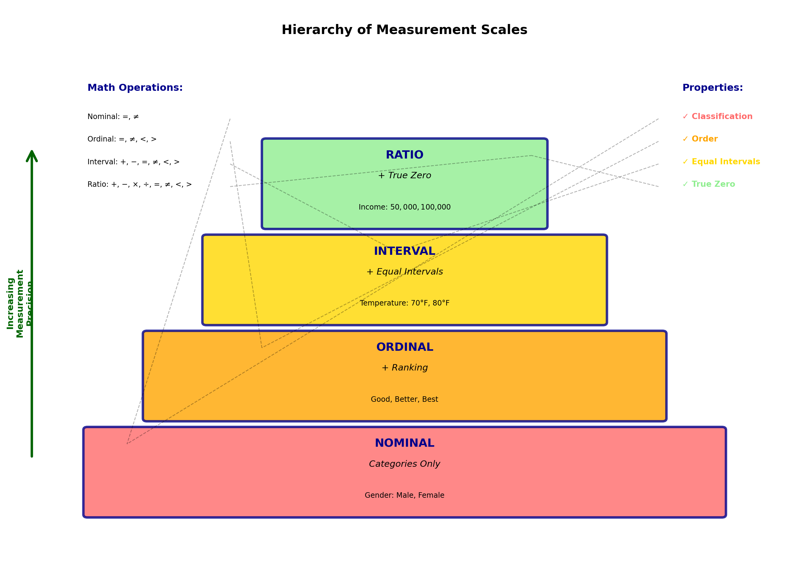
ImportantWhy Measurement Scales Matter
Choosing the right statistical method depends on the measurement scale:
Nominal data:
✗ Cannot calculate mean (what is “average gender”?)
✓ Can calculate mode (most common category)
Ordinal data:
✗ Cannot meaningfully add ranks
✓ Can find median rank
Interval data:
✗ Cannot say “twice as much”
✓ Can calculate means and standard deviations
Ratio data:
✓ All operations valid
✓ Most flexible for analysis
Common mistake: Treating ordinal data as interval data (e.g., averaging Likert scale responses without justification).
2.8 1.7 Chapter Summary
This chapter introduced the fundamental concepts that form the foundation of statistical thinking and analysis.
2.8.1 Key Concepts Review
1. Importance of Statistics in Business
- Essential tool for data-driven decision making
- Provides framework for managing uncertainty
- Enables prediction and forecasting
- Supports quality control and process improvement
2. Fundamental Definitions
- Population: Complete collection of all observations (parameter \mu, \sigma, p)
- Sample: Subset selected for study (statistic \bar{x}, s, \hat{p})
- Variables: Characteristics being measured (quantitative/qualitative, continuous/discrete)
3. Branches of Statistics
- Descriptive Statistics: Organizing, summarizing, presenting data
- Inferential Statistics: Using samples to draw conclusions about populations
- Sampling Error: Inevitable difference between statistic and parameter
4. Functions of Statistics
- Collection → Organization → Presentation → Analysis → Interpretation
- Continuous cycle of improvement
- Supports every aspect of business operations
5. Measurement Scales
- Nominal: Categories without order (Gender, Product type)
- Ordinal: Categories with order (Good/Better/Best)
- Interval: Numeric with arbitrary zero (Temperature °F)
- Ratio: Numeric with true zero (Income, Weight)
2.8.2 Looking Ahead
The concepts introduced in this chapter provide the language and framework for everything that follows. In the next chapters, we will:
- Chapter 2: Learn how to organize and summarize data using tables and graphs
- Chapter 3: Calculate descriptive measures (mean, median, standard deviation)
- Chapters 4-6: Understand probability and probability distributions
- Chapters 7-9: Master inferential statistics (estimation and hypothesis testing)
- Later chapters: Apply these tools to regression, ANOVA, quality control, and more
TipStudy Tips for Success
1. Master the vocabulary
- Know the difference between population and sample
- Understand parameter vs. statistic
- Recognize measurement scales in examples
2. Think in context
- Always ask: “What is the population?”
- Consider: “Is this sample representative?”
- Question: “What scale of measurement applies?”
3. Connect to business applications
- See statistics as a business tool, not just math
- Relate concepts to real-world decisions
- Practice with business examples
4. Build on fundamentals
- These concepts recur throughout the course
- Each chapter builds on previous knowledge
- Understanding Chapter 1 makes everything easier
Statistics is not just about calculations—it’s about thinking clearly about data, understanding uncertainty, and making better decisions. The journey begins with these fundamental concepts.
2.9 Glossary of Key Terms
Continuous Variable: A variable that can take any value within a range; usually results from measurement.
Descriptive Statistics: Methods for organizing, summarizing, and presenting data in an informative way.
Discrete Variable: A variable limited to certain values, usually integers; often results from counting.
Inferential Statistics: Methods for using sample data to make generalizations about a larger population.
Interval Scale: Measurements on a numerical scale where zero is arbitrary but differences are meaningful.
Nominal Scale: Names or classifications for distinct categories without inherent order.
Ordinal Scale: Classifications with a meaningful order but unequal intervals.
Parameter: A descriptive measure of a population (usually unknown).
Population: The complete collection of all observations of interest.
Qualitative Variable: A variable measured in non-numerical terms (categories).
Quantitative Variable: A variable that can be expressed numerically.
Ratio Scale: The highest level of measurement with a true zero point; both differences and ratios are meaningful.
Sample: A representative subset of a population selected for study.
Sample Bias: Systematic tendency to favor selection of certain elements over others.
Sampling Error: The difference between a sample statistic and the unknown population parameter.
Statistic: A descriptive measure of a sample used to estimate a population parameter.
Variable: A characteristic of a population or sample being analyzed in a statistical study.
This completes Chapter 1. You now have the foundational concepts needed to begin your statistical journey!